吴恩达团队 Tensorflow课程学习笔记 5

利用keras使用图片生成器来自动载入并基于目录为文件打标签来创建一个神经网络,构建人马分类器

准备数据集

考虑数据集不均匀的情况(更接近实际情况)，首先下载包含马和人的数据的压缩文件

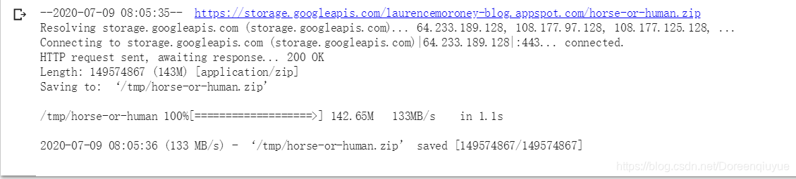
下载图片

下载文件的代码

!wget --no-check-certificate \
    https://storage.googleapis.com/laurencemoroney-blog.appspot.com/horse-or-human.zip \
    -O /tmp/horse-or-human.zip

解压压缩文件

解压到这个虚拟机的缓存目录

import os #使用os库来使用操作系统库，从而可以访问文件系统
import zipfile #解压数据

local_zip = '/tmp/horse-or-human.zip'
zip_ref = zipfile.ZipFile(local_zip, 'r')
zip_ref.extractall('/tmp/horse-or-human')
zip_ref.close()

zip文件包含两个子目录，解压后就已经创建好了

# Directory with our training horse pictures
train_horse_dir = os.path.join('/tmp/horse-or-human/horses')

# Directory with our training human pictures
train_human_dir = os.path.join('/tmp/horse-or-human/humans')

浏览文件

train_horse_names = os.listdir(train_horse_dir)
print(train_horse_names[:10])

train_human_names = os.listdir(train_human_dir)
print(train_human_names[:10])

[‘horse34-9.png’, ‘horse33-0.png’, ‘horse31-9.png’, ‘horse27-7.png’, ‘horse06-1.png’, ‘horse50-5.png’, ‘horse21-9.png’, ‘horse36-1.png’, ‘horse18-2.png’, ‘horse02-4.png’]
[‘human10-26.png’, ‘human04-24.png’, ‘human16-06.png’, ‘human17-25.png’, ‘human04-13.png’, ‘human04-28.png’, ‘human16-22.png’, ‘human07-23.png’, ‘human17-05.png’, ‘human13-09.png’]
可用于生成标签，但是如果用keras生成器的话就不需要了

打印参与训练的图片数量

print('total training horse images:', len(os.listdir(train_horse_dir)))
print('total training human images:', len(os.listdir(train_human_dir)))

total training horse images: 500
total training human images: 527

在数据集随机展示小部分图片

设置matplot参数

%matplotlib inline

import matplotlib.pyplot as plt
import matplotlib.image as mpimg

# Parameters for our graph; we'll output images in a 4x4 configuration
nrows = 4
ncols = 4

# Index for iterating over images
pic_index = 0

展示图片

# Set up matplotlib fig, and size it to fit 4x4 pics
fig = plt.gcf()
fig.set_size_inches(ncols * 4, nrows * 4)

pic_index += 8
next_horse_pix = [os.path.join(train_horse_dir, fname) 
                for fname in train_horse_names[pic_index-8:pic_index]]
next_human_pix = [os.path.join(train_human_dir, fname) 
                for fname in train_human_names[pic_index-8:pic_index]]

for i, img_path in enumerate(next_horse_pix+next_human_pix):
  # Set up subplot; subplot indices start at 1
  sp = plt.subplot(nrows, ncols, i + 1)
  sp.axis('Off') # Don't show axes (or gridlines)

  img = mpimg.imread(img_path)
  plt.imshow(img)

plt.show()

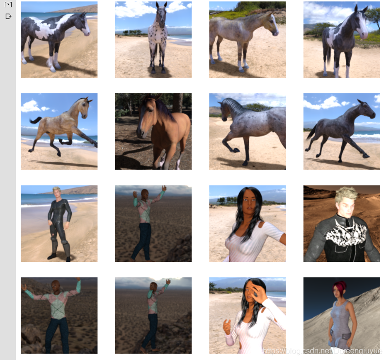
这里有8匹马和8个人，这个数据集的所有图片都是计算机生成的

Tensorflow中的图片生成器

特性

指向一个目录，然后它的子目录自动生成标签

考虑上面这个目录结构，图像目录下有训练和验证的子目录，当把马和人的子目录放在这些目录中，并在其中存储必要图像时，图片生成器可以为这些图片创建一个Feeder，并且为你自动标记。
例如，在训练目录指向一个图片生成器，标签将是马和人，并且每个目录中的图片将会加载并且相应标记。

实例化一个生成器

from tensorflow.keras.preprocessing.image import ImageDataGenerator

train_datagen = ImageDataGenerator(rescale=1./255) #将rescale传递给生成器，使其数据标准化，将个像素值转化到0-1之间

#调用目录流方法，从该目录及其子目录加载图像，常见的错误是把子目录指向生成器
#应该始终将其指向包含你的图像的子目录的那个目录，子目录的名称将是它包含的图片的标签
train_generator = train_datagen.flow_from_directory(
        train_dir, #指向的目录
        target_size=(300,300), #需要将图片调成一致，不影响源数据，不需要自己动手处理
        batch_size=128, #批次载入，有一个完整的科学计算批次大小这里暂不讨论
        class_mode='binary') #分类模型
 
#验证生成器
test_datagen = ImageDataGenerator(rescale=1./255)
validation_generator = test_datagen.flow_from_directory(
        validation_dir, #指向的目录
        target_size=(300,300), #需要将图片调成一致，不影响源数据
        batch_size=32, #批次载入
        class_mode='binary') #分类模型

设计神经网络

构建模型

模型采用顺序排列
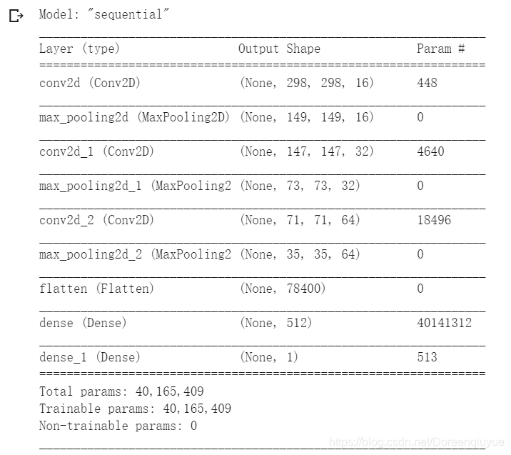
这次图片的清晰度高，(300*300)，所以进行了三次压缩

model = tf.keras.models.Sequential([
    tf.keras.layers.Conv2D(16,(3,3),activation='relu',
                           input_shape=(300,300,3)),  #彩色图片
    tf.keras.layers.MaxPooling2D(2,2),
    tf.keras.layers.Conv2D(32,(3,3),activation='relu'),
    tf.keras.layers.MaxPooling2D(2,2),
    tf.keras.layers.Conv2D(64,(3,3),activation='relu'),
    tf.keras.layers.MaxPooling2D(2,2),
    tf.keras.layers.Flatten(),
    tf.keras.layers.Dense(512,activation='relu'),
    tf.keras.layers.Dense(1,activation='sigmoid')  #输出神经元个数为1个，因为输出函数是sigmoid，用于二分类。
])

模型结构展示

编译模型

from tensorflow.keras.optimizers import RMSprop

model.compile(loss='binary_crossentropy', #二值交叉熵(二分类)
              optimizer=RMSprop(lr=0.001), #可以调整学习率
              metrics=['acc'])

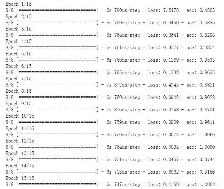
模型训练代码

#使用的生成器来调用数据集，所以调用的model.fit_generator
history = model.fit_generator( 
      train_generator, #之前设置的训练生成器，从训练目录中流式传输图像，创建它的时候使用的批量大小是20，不太懂??
      steps_per_epoch=8, #训练目录里有1024张图片，所以每次载入128个，分8批
      epochs=15,
      validation_data=validation_generator,
      validation_steps=8, #验证集有256张图片，每次载入32个，分8批
      verbose=2) #verbose指定当训练继续时显示多少，获取隐藏在epoch过程的动画

模型训练过程展示

模型测试代码

import numpy as np
from google.colab import files
from keras.preprocessing import image

uploaded = files.upload()

#循环遍历集合中所有的图像
for fn in uploaded.keys():
  path = '/content/' + fn
  img = image.load_img(path,target_size=(300,300)) #注意尺寸的匹配
  x = image.img_to_array(img)
  x = np.expand_dims(x,axis=0)

images = np.vstack([x])
classes = model.predict(images,batch_size=10) #调用model.predict，它会返回分类数组，在二分类的情况下，它只包含一个值，一个类的值接近0，另一个类的值接近1
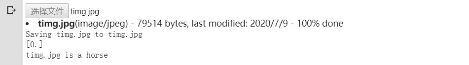
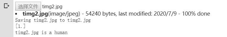
print(classes[0])
if classes[0]>0.5:
  print(fn + "is a human")
else:
  print(fn + "is a horse")

测试结果

①测试的第一幅图像及结果

②测试的第二幅图像及结果

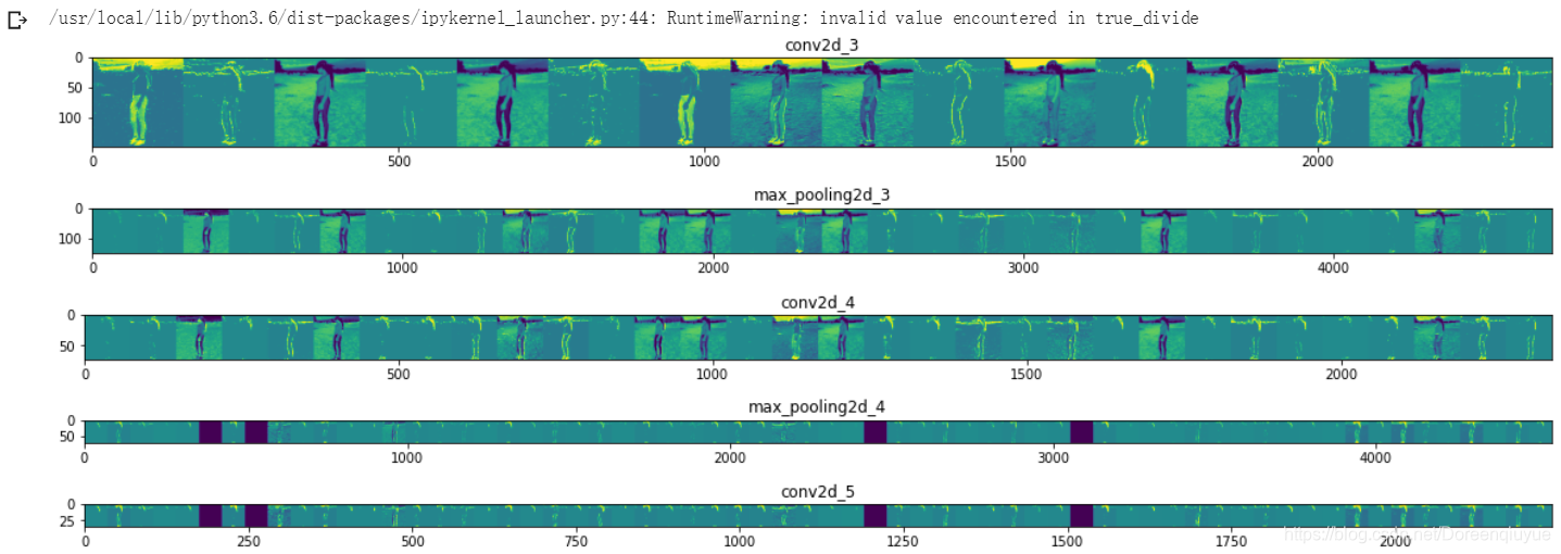
卷积过程的可视化

import numpy as np
import random
from tensorflow.keras.preprocessing.image import img_to_array, load_img

# Let's define a new Model that will take an image as input, and will output
# intermediate representations for all layers in the previous model after
# the first.
successive_outputs = [layer.output for layer in model.layers[1:]]
#visualization_model = Model(img_input, successive_outputs)
visualization_model = tf.keras.models.Model(inputs = model.input, outputs = successive_outputs)
# Let's prepare a random input image from the training set.
horse_img_files = [os.path.join(train_horse_dir, f) for f in train_horse_names]
human_img_files = [os.path.join(train_human_dir, f) for f in train_human_names]
img_path = random.choice(horse_img_files + human_img_files)

img = load_img(img_path, target_size=(300, 300))  # this is a PIL image
x = img_to_array(img)  # Numpy array with shape (150, 150, 3)
x = x.reshape((1,) + x.shape)  # Numpy array with shape (1, 150, 150, 3)

# Rescale by 1/255
x /= 255

# Let's run our image through our network, thus obtaining all
# intermediate representations for this image.
successive_feature_maps = visualization_model.predict(x)

# These are the names of the layers, so can have them as part of our plot
layer_names = [layer.name for layer in model.layers]

# Now let's display our representations
for layer_name, feature_map in zip(layer_names, successive_feature_maps):
  if len(feature_map.shape) == 4:
    # Just do this for the conv / maxpool layers, not the fully-connected layers
    n_features = feature_map.shape[-1]  # number of features in feature map
    # The feature map has shape (1, size, size, n_features)
    size = feature_map.shape[1]
    # We will tile our images in this matrix
    display_grid = np.zeros((size, size * n_features))
    for i in range(n_features):
      # Postprocess the feature to make it visually palatable
      x = feature_map[0, :, :, i]
      x -= x.mean()
      x /= x.std()
      x *= 64
      x += 128
      x = np.clip(x, 0, 255).astype('uint8')
      # We'll tile each filter into this big horizontal grid
      display_grid[:, i * size : (i + 1) * size] = x
    # Display the grid
    scale = 20. / n_features
    plt.figure(figsize=(scale * n_features, scale))
    plt.title(layer_name)
    plt.grid(False)
    plt.imshow(display_grid, aspect='auto', cmap='viridis')