


目录
人和马的分类及可视化隐藏层
内容总结自吴恩达TensorFlow2.0的课程
数据处理
下载数据集
注意路径要写的是绝对路径,而且需要事先安装wget。
!wget --no-check-certificate \
    https://storage.googleapis.com/laurencemoroney-blog.appspot.com/horse-or-human.zip \
    -O /tmp/horse-or-human.zip
    !wget --no-check-certificate \
    https://storage.googleapis.com/laurencemoroney-blog.appspot.com/validation-horse-or-human.zip \
    -O /tmp/validation-horse-or-human.zip
如果命令执行不了的,可以点击这里下载训练集和验证集。虽然是谷歌的数据但是好像不需要科学上网。
解压数据集
import os
import zipfile
base = 'C:/Users/学习/吴恩达tf2.0/dlaicourse-master'
local_zip = base + '/tmp/horse-or-human.zip'
# 以读的方式打开压缩文件
# r读,w写,x创建一个新的并且写入,a在后面添加
zip_ref = zipfile.ZipFile(local_zip, 'r')
# 解压到指定位置
zip_ref.extractall(base + '/tmp/horse-or-human')
local_zip = base + '/tmp/validation-horse-or-human.zip'
zip_ref = zipfile.ZipFile(local_zip, 'r')
zip_ref.extractall(base + '/tmp/validation-horse-or-human')
zip_ref.close()
确定路径
# 指定每一种数据的位置
# Directory with our training horse pictures
train_horse_dir = os.path.join(base + '/tmp/horse-or-human/horses')

# Directory with our training human pictures
train_human_dir = os.path.join(base + '/tmp/horse-or-human/humans')

# Directory with our training horse pictures
validation_horse_dir = os.path.join(base + '/tmp/validation-horse-or-human/horses')

# Directory with our training human pictures
validation_human_dir = os.path.join(base + '/tmp/validation-horse-or-human/humans')
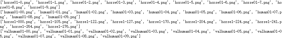
打印数据名
# os.listdir返回所给路径下的所有文件名的列表
train_horse_names = os.listdir(train_horse_dir)
print(train_horse_names[:10])

train_human_names = os.listdir(train_human_dir)
print(train_human_names[:10])

validation_horse_hames = os.listdir(validation_horse_dir)
print(validation_horse_hames[:10])

validation_human_names = os.listdir(validation_human_dir)
print(validation_human_names[:10])
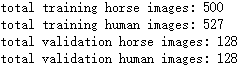
获取每种数据的数量
print('total training horse images:', len(os.listdir(train_horse_dir)))
print('total training human images:', len(os.listdir(train_human_dir)))
print('total validation horse images:', len(os.listdir(validation_horse_dir)))
print('total validation human images:', len(os.listdir(validation_human_dir)))
数据集可视化
引入头文件
%matplotlib inline

import matplotlib.pyplot as plt
import matplotlib.image as mpimg

# 设置我们要画的图的参数
nrows = 4
ncols = 4

# 我们要选择进行可视化的数据集的起始位置
pic_index = 0
绘图
# 设置图片为4行4列,图片大小为16x16
fig, ax = plt.subplots(nrows=4, ncols=4, figsize=(4 * nrows, 4 * ncols))
# 选定我们要画的图片的位置
pic_index += 8
# 读取图片的地址
next_horse_pix = [os.path.join(train_horse_dir, fname)
                for fname in train_horse_names[pic_index-8:pic_index]]
next_human_pix = [os.path.join(train_human_dir, fname)
                for fname in train_human_names[pic_index-8:pic_index]]
# 用枚举类型进行遍历
for i, img_path in enumerate(next_horse_pix+next_human_pix):
  # 这里注意图片是4x4的。画图时不能用ax[1].imshow
  img = mpimg.imread(img_path)
  ax[int(i/4),i%4].imshow(img)
  ax[int(i/4),i%4].axis('Off')

设计训练模型
引入头文件
import tensorflow as tf
设计模型
model = tf.keras.models.Sequential([
    # 我们的数据是300x300而且是三通道的,所以我们的输入应该设置为这样的格式。
    # This is the first convolution
    tf.keras.layers.Conv2D(16, (3,3), activation='relu', input_shape=(300, 300, 3)),
    tf.keras.layers.MaxPooling2D(2, 2),
    # The second convolution
    tf.keras.layers.Conv2D(32, (3,3), activation='relu'),
    tf.keras.layers.MaxPooling2D(2,2),
    # The third convolution
    tf.keras.layers.Conv2D(64, (3,3), activation='relu'),
    tf.keras.layers.MaxPooling2D(2,2),
    # The fourth convolution
    tf.keras.layers.Conv2D(64, (3,3), activation='relu'),
    tf.keras.layers.MaxPooling2D(2,2),
    # The fifth convolution
    tf.keras.layers.Conv2D(64, (3,3), activation='relu'),
    tf.keras.layers.MaxPooling2D(2,2),
    # Flatten the results to feed into a DNN
    tf.keras.layers.Flatten(),
    # 512 neuron hidden layer
    tf.keras.layers.Dense(512, activation='relu'),
    # 因为是2分类所以只需要一个输出。
    tf.keras.layers.Dense(1, activation='sigmoid')
])
打印模型相关信息
model.summary()

进行优化方法选择和一些超参数设置
from tensorflow.keras.optimizers import RMSprop
# 因为只有两个分类。所以用2分类的交叉熵,使用RMSprop,学习率为0.001.优化指标为accuracy
model.compile(loss='binary_crossentropy',
              optimizer=RMSprop(lr=0.001),
              metrics=['acc'])
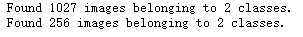
数据处理(利用ImageDataGenerator自动打标签)
因为我们的读取数据的时候不一定有标签,我们可以通过将图片放在不同的路径下的方式,来让ImageDataGenerator替我们自动打好标签。
from tensorflow.keras.preprocessing.image import ImageDataGenerator

# 把每个数据都放缩到0到1范围内
train_datagen = ImageDataGenerator(rescale=1/255)
validation_datagen = ImageDataGenerator(rescale=1/255)

# 生成训练集的带标签的数据
train_generator = train_datagen.flow_from_directory(
        base + '/tmp/horse-or-human/',  # 训练图片的位置
        target_size=(300, 300),  # 将图片统一大小
        batch_size=128, # 每一个投入多少张图片训练
        # 设置我们需要的标签类型
        class_mode='binary')

# 生成验证集带标签的数据
validation_generator = validation_datagen.flow_from_directory(
        base + '/tmp/validation-horse-or-human/',  # 训练图片的位置
        target_size=(300, 300),  # 将图片统一大小
        batch_size=32,
        # 设置我们需要的标签类型
        class_mode='binary')
进行训练
history = model.fit_generator( # 这里用的不是一般的fit
      train_generator,
      steps_per_epoch=8,
      epochs=15,
      verbose=1,
      validation_data = validation_generator,
      validation_steps=8)

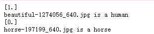
使用我们自己的图片进行验证
这里随便从网上找几张照片放在base+’/tmp/content/'的目录下即可。我的图片是从这个网站下载的。
import numpy as np
from keras.preprocessing import image
filePath = base + '/tmp/content/'
keys = []
# 获取所有文件名
for i,j,k in os.walk(filePath):
    keys = k
for fn in keys:
  # 对图片进行预测
  # 读取图片
  path = base + '/tmp/content/' + fn
  img = image.load_img(path, target_size=(300, 300))
  x = image.img_to_array(img)
  # 在第0维添加维度变为1x300x300x3,和我们模型的输入数据一样
  x = np.expand_dims(x, axis=0)
  # np.vstack:按垂直方向(行顺序)堆叠数组构成一个新的数组,我们一次只有一个数据所以不这样也可以
  images = np.vstack([x])
  # batch_size批量大小,程序会分批次地预测测试数据,这样比每次预测一个样本会快。因为我们也只有一个测试所以不用也可以
  classes = model.predict(images, batch_size=10)
  print(classes[0])
  if classes[0]>0.5:
    print(fn + " is a human")
  else:
    print(fn + " is a horse")
可视化隐藏层
import numpy as np
import random
from tensorflow.keras.preprocessing.image import img_to_array, load_img


# 让我们定义一个新模型,该模型将图像作为输入,并输出先前模型中所有层的中间表示。
successive_outputs = [layer.output for layer in model.layers[1:]]
# 进行可视化模型搭建,设置输入和输出
visualization_model = tf.keras.models.Model(inputs = model.input, outputs = successive_outputs)
# 选取一张随机的图片
horse_img_files = [os.path.join(train_horse_dir, f) for f in train_horse_names]
human_img_files = [os.path.join(train_human_dir, f) for f in train_human_names]
img_path = random.choice(horse_img_files + human_img_files)  # 随机选取一个

img = load_img(img_path, target_size=(300, 300))  # 以指定大小读取图片
x = img_to_array(img)  # 变成array
x = x.reshape((1,) + x.shape)  # 变成 (1, 300, 300, 3)

# 统一范围到0到1
x /= 255

# 运行我们的模型,得到我们要画的图。
successive_feature_maps = visualization_model.predict(x)

# 选取每一层的名字
layer_names = [layer.name for layer in model.layers]

# 开始画图
for layer_name, feature_map in zip(layer_names, successive_feature_maps):
  if len(feature_map.shape) == 4:
    # 只绘制卷积层,池化层,不画全连接层。
    n_features = feature_map.shape[-1]  # 最后一维的大小,也就是通道数,也是我们提取的特征数
    # feature_map的形状为 (1, size, size, n_features)
    size = feature_map.shape[1]
    # 我们将在此矩阵中平铺图像
    display_grid = np.zeros((size, size * n_features))
    for i in range(n_features):
      # 后期处理我们的特征,使其看起来更美观。
      x = feature_map[0, :, :, i]
      x -= x.mean()
      x /= x.std()
      x *= 64
      x += 128
      x = np.clip(x, 0, 255).astype('uint8')
      # 我们把图片平铺到这个大矩阵中
      display_grid[:, i * size : (i + 1) * size] = x
    # 绘制这个矩阵
    scale = 20. / n_features
    plt.figure(figsize=(scale * n_features, scale))  # 设置图片大小
    plt.title(layer_name)  # 设置题目
    plt.grid(False)  # 不绘制网格线
    # aspect='auto'自动控制轴的长宽比。 这方面对于图像特别相关,因为它可能会扭曲图像,即像素不会是正方形的。
    # cmap='viridis'设置图像的颜色变化
    plt.imshow(display_grid, aspect='auto', cmap='viridis')

终止程序
结束程序释放资源。signal模块可以在linux下正常使用,但在windows下却有一些限制。好像不能正常运行。
import os, signal
os.kill(os.getpid(), signal.SIGKILL)


 332
332


 被折叠的 条评论
为什么被折叠?
被折叠的 条评论
为什么被折叠?
 到【灌水乐园】发言


