GC-Net 笔记及探讨 --- unary特征以及级联的cost volume （更新中）

FLOWVERSE

已于 2022-02-08 16:53:37 修改

阅读量2.2k

点赞数 10

分类专栏：深度学习与机器学习 # 基于深度学习的立体匹配文章标签：深度学习计算机视觉人工智能

于 2021-03-23 10:25:18 首次发布

本文链接：https://blog.csdn.net/flow_specter/article/details/115049928

版权

基于深度学习的立体匹配同时被 2 个专栏收录

15 篇文章 26 订阅

订阅专栏

深度学习与机器学习

9 篇文章 2 订阅

订阅专栏

文章目录

前言
论文结构
3.1 Unary Feature 笔记
3.2 Cost Volume 笔记及衍生
附录

前言

读比较新的AANet，patchmatch-net等等各种fancy的net的时候，总是会不停的往前追溯，总会追溯到GC-net，借鉴到GC-net的思想。因此，决定精读GC-Net，并做以下笔记。

论文结构

基于深度学习的cost volume构建思想，其实许多文章中所采用的构建方式就来源于这篇GC-Net。
在看网络结构之前，先看看论文结构吧。

Introduction
Related Work
Learning End-to-end Disparity Regression
3.1 Unary Features
3.2 Cost Volume
3.3 Learning Context
3.4 Differentiable ArgMin
3.5 Loss
Experimental Evaluation
4.1 Model Design Analysis
4.2 KITTI Benchmark
4.3 Model Saliency(模型特点)
Conclusions
在后来的文章里，经常会看到3.1 unary Features以及3.2 Cost volume。因此，先来精读3.1以及3.2。

3.1 Unary Feature 笔记

在这里插入图片描述
为了计算立体匹配的代价，需要去学习一些深度表达。不像传统方法那样，直接使用影像的灰度值，而是去使用经过变换过的特征表达。为什么说利用特征表达比直接用影像的灰度值要好呢？因为这样往往更加的鲁棒，而且还能够隐含一些些邻域信息。
为了学习深度表达，使用了一定数量的二维卷积操作。每一个卷积都跟着一个BN层以及一个ReLU层，记得吗，这在patchmatch-net的源码中出现过，封装成了ConvBnRelu层（参考链接）。为了降低计算需求，先是应用了核稍显大一点的一个 $5\times 5$ 的卷积核以及stride为2来对输入的图像进行采样。紧接着是8个residual blocks(每个residual block都包含着两个3 *3 大小的卷积核)。最终，得到属于左右影像的两纵溜儿的特征。

3.2 Cost Volume 笔记及衍生

在这里插入图片描述

在3.1中，已经拿到了对应左右影像的两纵溜儿的特征(个数分别为F)，现在应该怎么通过这些特征来构建代价空间呢？在传统方法中，构建代价空间的方式是固定左影像，然后对右影像根据预先设定的视差范围进行shift，然后与左影像进行某个操作，比如说AD，来得到属于这个视差的每一个平面像素的代价值，这一层代价值被压到代价空间的最底下（d=min_disp），然后一层一层的叠加后（d=min_disp+1,…,max_disp），就形成了视差空间。
其实2018 CVPR的psm-net的cost volume也是借鉴了GC-Net的特征级联的方式，具体的实现代码好像更好理解一些，具体为：

        #matching
        cost = Variable(torch.FloatTensor(refimg_fea.size()[0], refimg_fea.size()[1]*2, self.maxdisp/4,  refimg_fea.size()[2],  refimg_fea.size()[3]).zero_(), volatile= not self.training).cuda()

        for i in range(self.maxdisp/4):
            if i > 0 :
             cost[:, :refimg_fea.size()[1], i, :,i:]   = refimg_fea[:,:,:,i:]
             cost[:, refimg_fea.size()[1]:, i, :,i:] = targetimg_fea[:,:,:,:-i]
            else:
             cost[:, :refimg_fea.size()[1], i, :,:]   = refimg_fea
             cost[:, refimg_fea.size()[1]:, i, :,:]   = targetimg_fea
        cost = cost.contiguous()

上述代码中，refimg_fea就是左图的特征，targetimg_fea就是右图的特征。cost_volume的级联先是所有的左图的特征（带偏移），然后是右图的特征。比如对于左图的某个特征来说，cost[d,所有行，d列到最后一列] = 对应的左图特征[所有行，d列到最后一列]。也就是说对于第一个特征，视差图就是它的逐个偏移，然后这样级联下去。这就很好理解，但是这好像和上述的GC-net的结果不同，先看这个的示意图：
在这里插入图片描述
上面的示意图主要针对的是左图的特征的cost volume 构建，右图稍有些区别，cost[:, refimg_fea.size()[1]:, i, :,i:] = targetimg_fea[:,:,:,:-i]，现在以右图中的某一个特征为例，有cost[某视差，所有行，视差列到最后一列]=右图对应特征[所有行，第一列到某视差列]，即相当于对右边的特征来说，是右边补0。想一想，如果对于右边的特征也往右边进行平移的话，那么重叠部分就会越来越少，所以，为了重叠，要对于右边的特征取左边的部分。以下是我画的示意图，说明了对于某一对左右特征图来说，在 $d = 1$ 的情况下的平移操作以及该视差下的cost volume的样子。 $d$ 在所有候选视差下都构成这样的切面，将这些切面叠在一起，就形成了属于某个特征的视差空间，或者说属于某个特征的cost volume。经由这样的操作，可以得到一个四维的cost volume（一共2F个特征），后续的三维卷积是对于每一个3D的cost volume在其height、width以及视差维进行的卷积，然后再将这一共2F个各个特征的视差空间的卷积结果进行加和，得到一个对四维cost volume的三维卷积结果，也因此相当于集合了特征维的信息，假设三维卷积不改变某个特征的三维空间的长宽高，一个三维卷积则说明输出的是一个三维体，而有10个三维卷积，则说明输出是十个卷积后的三维体。（个人理解，如果有误，望指出）

在这里插入图片描述

再接着去看在GC-Net中是怎么构建代价空间的。从上面也看出来了，这种级联的代价空间和我们传统方法中所认知的代价空间有些出入，其代价空间或许称作为特征空间更合适，因为它其实并不怎么体现相似性的测度。
主要在github上找到了两份gc-net实现中的cost_volume代码，一份来自于链接：

    def cost_volume(self,imgl,imgr):
        B, C, H, W = imgl.size()
        cost_vol = torch.zeros(B, C * 2, self.maxdisp , H, W).type_as(imgl)
        for i in range(self.maxdisp):
            if i > 0:
                cost_vol[:, :C, i, :, i:] = imgl[:, :, :, i:]
                cost_vol[:, C:, i, :, i:] = imgr[:, :, :, :-i]
            else:
                cost_vol[:, :C, i, :, :] = imgl
                cost_vol[:, C:, i, :, :] = imgr
        return cost_vol

与psm-net的想法基本一致，就不赘述了。
其实这样的级联cost volume实现应该是比较权威和受认可的，因为在gwc-net的实现中，也见到了这样的实现，可读性更强（也有可能是因为gwc-net就是在psm-net的基础上改进而来的…）：

def build_concat_volume(refimg_fea, targetimg_fea, maxdisp):
    B, C, H, W = refimg_fea.shape
    volume = refimg_fea.new_zeros([B, 2 * C, maxdisp, H, W])
    for i in range(maxdisp):
        if i > 0:
            volume[:, :C, i, :, i:] = refimg_fea[:, :, :, i:]
            volume[:, C:, i, :, i:] = targetimg_fea[:, :, :, :-i]
        else:
            volume[:, :C, i, :, :] = refimg_fea
            volume[:, C:, i, :, :] = targetimg_fea
    volume = volume.contiguous()
    return volume

但是我看到了另外一个从github上扒下来的开源代码，个人添加了一些注释。之后，还给出了一个小例子来试图诠释这个函数，但是，最终的结果，好像上面psm-net的级联的结果不一样，或许是在重组打包的过程中出了差错，也可能是本来就不一样，我暂时还没有想清楚，如果有了解的同学，望不吝指教。

    def cost_volume(self,imgl,imgr):
        xx_list = []
        # 向右padding最大视差距离的0
        pad_opr1 = nn.ZeroPad2d((0, self.maxdisp, 0, 0))
        xleft = pad_opr1(imgl) # 现在xleft的右边补上了maxdisp距离的0
        # 视差的范围是0到maxdisp。左闭右开，应该是maxdisp
        for d in range(self.maxdisp):  # maxdisp+1 ?
        	# 将右影像的左边补上d个0，相当于将右影像往右平移了d个位置，也即，视差为d，而往右paddingmaxdisp-d则是为了使得影像大小与左影像一样大。
            pad_opr2 = nn.ZeroPad2d((d, self.maxdisp - d, 0, 0))
            xright = pad_opr2(imgr)
            # 直接向右边连接了，比如两个两行三列的影像，这样cat后的结果是两行六列/
            xx_temp = torch.cat((xleft, xright), 1)
            # 将属于这个d的cat结果加进列表中。列表的每一个元素都是一个对应d的左右影像连接二维图
            xx_list.append(xx_temp)
        # 如果总共有n个候选的d，padding后的影像为w*h,那么这里xx的纬度应该是(w*d) * h    
        xx = torch.cat(xx_list, 1)
        # xx的纬度重组为5维，分别是1，最大视差，64，影像高的一半，影像宽的一半与最大视差的加和
        xx = xx.view(1, self.maxdisp, 64, int(self.height / 2), int(self.width / 2) + self.maxdisp)
        # 重组维度，分别是1，64（=2F,由于论文中的F，即特征数量是32，所以这里的维度直接定成了64），最大视差，影像高的一半，影像宽的一半与最大视差的加和
        xx0=xx.permute(0,2,1,3,4)
        # 视差空间的宽截断为影像的宽的一半
        xx0 = xx0[:, :, :, :, :int(self.width / 2)]
        return xx0

可能现在看完代码以及文字描述后还是弄不清细节。现在举一些例子来辅助说明。
首先，模拟左右的分别的两个特征作为输入。两张特征图的高是4，宽是5，特征的数量是3，由torch的rand函数构建：

import torch
import torch.nn as nn
import torch.nn.functional as F 
# 通道，高，宽，三张4*5大小的图片，每张是一个特征图
# 模拟左右特征输入
simu_left_feat = torch.rand((3,4,5)) 
simu_right_feat = torch.rand((3,4,5))
print(simu_left_feat)
print(simu_right_feat)

输出为：

tensor([[[0.9845, 0.5348, 0.9081, 0.2348, 0.5561],
         [0.8853, 0.7792, 0.3764, 0.2872, 0.2274],
         [0.3899, 0.9534, 0.2604, 0.7559, 0.9430],
         [0.6001, 0.5894, 0.5838, 0.3656, 0.2829]],

        [[0.3588, 0.6924, 0.6452, 0.3960, 0.4911],
         [0.9899, 0.2663, 0.0148, 0.4319, 0.3196],
         [0.1989, 0.8821, 0.2148, 0.1900, 0.5446],
         [0.7638, 0.0016, 0.6632, 0.8193, 0.3424]],

        [[0.4859, 0.6421, 0.5830, 0.2791, 0.6929],
         [0.7707, 0.4133, 0.2004, 0.9595, 0.3127],
         [0.5609, 0.8365, 0.6555, 0.0246, 0.0777],
         [0.7681, 0.9491, 0.8666, 0.5506, 0.2245]]])
tensor([[[0.2995, 0.8519, 0.5041, 0.6641, 0.2525],
         [0.7725, 0.2445, 0.7097, 0.6442, 0.3425],
         [0.2805, 0.0568, 0.9701, 0.0506, 0.2685],
         [0.6132, 0.6742, 0.1079, 0.5940, 0.8110]],

        [[0.4489, 0.5536, 0.4991, 0.4602, 0.5077],
         [0.7407, 0.1764, 0.5554, 0.3521, 0.1952],
         [0.0890, 0.0975, 0.4903, 0.3953, 0.7551],
         [0.9664, 0.8638, 0.3217, 0.1699, 0.9905]],

        [[0.1478, 0.4001, 0.5453, 0.2033, 0.6080],
         [0.0421, 0.0246, 0.4427, 0.6430, 0.6821],
         [0.0054, 0.9888, 0.1999, 0.2217, 0.9569],
         [0.4540, 0.8931, 0.1656, 0.7561, 0.3945]]])

现在假设最大的视差为3。将左特征体进行padding：

imgl=simu_left_feat
imgr=simu_right_feat
maxdisp = 3
pad_opr1 = nn.ZeroPad2d((0, maxdisp, 0, 0))
xleft = pad_opr1(imgl)
print(xleft)

输出为：
在这里插入图片描述
可以看到，对于左特征体中的每张特征影像，都在右边补上了最大视差，即距离为3的数值0，此时，左特征体的size变为了 $\times 4 \times 8$ ，即每张特征图由原本的 $\times 5$ 大小变为了 $\times 8$ 。
现在，需要逐候选视差的构建代价空间，即cost volume.
显然，当最大视差为3的时候（默认最小视差为0），候选视差有 $d = 0$ , $d = 1$ , $d = 2$ , $d = 3$ 。
紧接着，

xx_list=[]
for d in range(4):
     print('d:',d)
     pad_opr2 = nn.ZeroPad2d((d, maxdisp - d, 0, 0))
     xright = pad_opr2(imgr)
     xx_temp = torch.cat((xleft, xright), 1)
     print(xx_temp.size())
     print(xx_temp)
     print('----------------------------------------------------------------------')
     xx_list.append(xx_temp)

以 $d = 1$ 为例，首先将右特征体的每一张特征图都对应的向右平移 $d = 1$ 个位置，以好和对应的左特征图对应起来，比如：
在这里插入图片描述
此时右特征体的size和左特征体一致，都是 $\times 4 \times 8$ 。那么，对于 $d = 1$ ，我们可以取得对应位置的左右的特征图，GC-net的想法是将这两个特征图级联起来，也即xx_temp = torch.cat((xleft, xright), 1)，xx_temp的结果如下所示：

torch.Size([3, 8, 8])
tensor([[[0.9845, 0.5348, 0.9081, 0.2348, 0.5561, 0.0000, 0.0000, 0.0000],
         [0.8853, 0.7792, 0.3764, 0.2872, 0.2274, 0.0000, 0.0000, 0.0000],
         [0.3899, 0.9534, 0.2604, 0.7559, 0.9430, 0.0000, 0.0000, 0.0000],
         [0.6001, 0.5894, 0.5838, 0.3656, 0.2829, 0.0000, 0.0000, 0.0000],
         [0.0000, 0.2995, 0.8519, 0.5041, 0.6641, 0.2525, 0.0000, 0.0000],
         [0.0000, 0.7725, 0.2445, 0.7097, 0.6442, 0.3425, 0.0000, 0.0000],
         [0.0000, 0.2805, 0.0568, 0.9701, 0.0506, 0.2685, 0.0000, 0.0000],
         [0.0000, 0.6132, 0.6742, 0.1079, 0.5940, 0.8110, 0.0000, 0.0000]],

        [[0.3588, 0.6924, 0.6452, 0.3960, 0.4911, 0.0000, 0.0000, 0.0000],
         [0.9899, 0.2663, 0.0148, 0.4319, 0.3196, 0.0000, 0.0000, 0.0000],
         [0.1989, 0.8821, 0.2148, 0.1900, 0.5446, 0.0000, 0.0000, 0.0000],
         [0.7638, 0.0016, 0.6632, 0.8193, 0.3424, 0.0000, 0.0000, 0.0000],
         [0.0000, 0.4489, 0.5536, 0.4991, 0.4602, 0.5077, 0.0000, 0.0000],
         [0.0000, 0.7407, 0.1764, 0.5554, 0.3521, 0.1952, 0.0000, 0.0000],
         [0.0000, 0.0890, 0.0975, 0.4903, 0.3953, 0.7551, 0.0000, 0.0000],
         [0.0000, 0.9664, 0.8638, 0.3217, 0.1699, 0.9905, 0.0000, 0.0000]],

        [[0.4859, 0.6421, 0.5830, 0.2791, 0.6929, 0.0000, 0.0000, 0.0000],
         [0.7707, 0.4133, 0.2004, 0.9595, 0.3127, 0.0000, 0.0000, 0.0000],
         [0.5609, 0.8365, 0.6555, 0.0246, 0.0777, 0.0000, 0.0000, 0.0000],
         [0.7681, 0.9491, 0.8666, 0.5506, 0.2245, 0.0000, 0.0000, 0.0000],
         [0.0000, 0.1478, 0.4001, 0.5453, 0.2033, 0.6080, 0.0000, 0.0000],
         [0.0000, 0.0421, 0.0246, 0.4427, 0.6430, 0.6821, 0.0000, 0.0000],
         [0.0000, 0.0054, 0.9888, 0.1999, 0.2217, 0.9569, 0.0000, 0.0000],
         [0.0000, 0.4540, 0.8931, 0.1656, 0.7561, 0.3945, 0.0000, 0.0000]]])

这一层级联起来的左右特征图xx_temp大小则变成了 $\times 8 \times 8$ ，即3个大小为 $\times 8$ 大的图像。
我们知道，这里的候选视差有4个，那么对于每一个候选视差，都有先基于 $d$ 的左右特征"对齐"，后级联的操作，也就会有4个 $\times 8 \times 8$ 的tensor 被压进xx_list。
对存在xx_list中的这些对应不同 $d$ 的tensor进行级联：

xx = torch.cat(xx_list,1)
print(xx.size())
print(xx)

输出的xx的大小为 $\times 32 \times 8$ (后面的代码都是在对xx进行拆分打包重组):

torch.Size([3, 32, 8])
tensor([[[0.9845, 0.5348, 0.9081, 0.2348, 0.5561, 0.0000, 0.0000, 0.0000],
         [0.8853, 0.7792, 0.3764, 0.2872, 0.2274, 0.0000, 0.0000, 0.0000],
         [0.3899, 0.9534, 0.2604, 0.7559, 0.9430, 0.0000, 0.0000, 0.0000],
         [0.6001, 0.5894, 0.5838, 0.3656, 0.2829, 0.0000, 0.0000, 0.0000],
         [0.2995, 0.8519, 0.5041, 0.6641, 0.2525, 0.0000, 0.0000, 0.0000],
         [0.7725, 0.2445, 0.7097, 0.6442, 0.3425, 0.0000, 0.0000, 0.0000],
         [0.2805, 0.0568, 0.9701, 0.0506, 0.2685, 0.0000, 0.0000, 0.0000],
         [0.6132, 0.6742, 0.1079, 0.5940, 0.8110, 0.0000, 0.0000, 0.0000],
         [0.9845, 0.5348, 0.9081, 0.2348, 0.5561, 0.0000, 0.0000, 0.0000],
         [0.8853, 0.7792, 0.3764, 0.2872, 0.2274, 0.0000, 0.0000, 0.0000],
         [0.3899, 0.9534, 0.2604, 0.7559, 0.9430, 0.0000, 0.0000, 0.0000],
         [0.6001, 0.5894, 0.5838, 0.3656, 0.2829, 0.0000, 0.0000, 0.0000],
         [0.0000, 0.2995, 0.8519, 0.5041, 0.6641, 0.2525, 0.0000, 0.0000],
         [0.0000, 0.7725, 0.2445, 0.7097, 0.6442, 0.3425, 0.0000, 0.0000],
         [0.0000, 0.2805, 0.0568, 0.9701, 0.0506, 0.2685, 0.0000, 0.0000],
         [0.0000, 0.6132, 0.6742, 0.1079, 0.5940, 0.8110, 0.0000, 0.0000],
         [0.9845, 0.5348, 0.9081, 0.2348, 0.5561, 0.0000, 0.0000, 0.0000],
         [0.8853, 0.7792, 0.3764, 0.2872, 0.2274, 0.0000, 0.0000, 0.0000],
         [0.3899, 0.9534, 0.2604, 0.7559, 0.9430, 0.0000, 0.0000, 0.0000],
         [0.6001, 0.5894, 0.5838, 0.3656, 0.2829, 0.0000, 0.0000, 0.0000],
         [0.0000, 0.0000, 0.2995, 0.8519, 0.5041, 0.6641, 0.2525, 0.0000],
         [0.0000, 0.0000, 0.7725, 0.2445, 0.7097, 0.6442, 0.3425, 0.0000],
         [0.0000, 0.0000, 0.2805, 0.0568, 0.9701, 0.0506, 0.2685, 0.0000],
         [0.0000, 0.0000, 0.6132, 0.6742, 0.1079, 0.5940, 0.8110, 0.0000],
         [0.9845, 0.5348, 0.9081, 0.2348, 0.5561, 0.0000, 0.0000, 0.0000],
         [0.8853, 0.7792, 0.3764, 0.2872, 0.2274, 0.0000, 0.0000, 0.0000],
         [0.3899, 0.9534, 0.2604, 0.7559, 0.9430, 0.0000, 0.0000, 0.0000],
         [0.6001, 0.5894, 0.5838, 0.3656, 0.2829, 0.0000, 0.0000, 0.0000],
         [0.0000, 0.0000, 0.0000, 0.2995, 0.8519, 0.5041, 0.6641, 0.2525],
         [0.0000, 0.0000, 0.0000, 0.7725, 0.2445, 0.7097, 0.6442, 0.3425],
         [0.0000, 0.0000, 0.0000, 0.2805, 0.0568, 0.9701, 0.0506, 0.2685],
         [0.0000, 0.0000, 0.0000, 0.6132, 0.6742, 0.1079, 0.5940, 0.8110]],

        [[0.3588, 0.6924, 0.6452, 0.3960, 0.4911, 0.0000, 0.0000, 0.0000],
         [0.9899, 0.2663, 0.0148, 0.4319, 0.3196, 0.0000, 0.0000, 0.0000],
         [0.1989, 0.8821, 0.2148, 0.1900, 0.5446, 0.0000, 0.0000, 0.0000],
         [0.7638, 0.0016, 0.6632, 0.8193, 0.3424, 0.0000, 0.0000, 0.0000],
         [0.4489, 0.5536, 0.4991, 0.4602, 0.5077, 0.0000, 0.0000, 0.0000],
         [0.7407, 0.1764, 0.5554, 0.3521, 0.1952, 0.0000, 0.0000, 0.0000],
         [0.0890, 0.0975, 0.4903, 0.3953, 0.7551, 0.0000, 0.0000, 0.0000],
         [0.9664, 0.8638, 0.3217, 0.1699, 0.9905, 0.0000, 0.0000, 0.0000],
         [0.3588, 0.6924, 0.6452, 0.3960, 0.4911, 0.0000, 0.0000, 0.0000],
         [0.9899, 0.2663, 0.0148, 0.4319, 0.3196, 0.0000, 0.0000, 0.0000],
         [0.1989, 0.8821, 0.2148, 0.1900, 0.5446, 0.0000, 0.0000, 0.0000],
         [0.7638, 0.0016, 0.6632, 0.8193, 0.3424, 0.0000, 0.0000, 0.0000],
         [0.0000, 0.4489, 0.5536, 0.4991, 0.4602, 0.5077, 0.0000, 0.0000],
         [0.0000, 0.7407, 0.1764, 0.5554, 0.3521, 0.1952, 0.0000, 0.0000],
         [0.0000, 0.0890, 0.0975, 0.4903, 0.3953, 0.7551, 0.0000, 0.0000],
         [0.0000, 0.9664, 0.8638, 0.3217, 0.1699, 0.9905, 0.0000, 0.0000],
         [0.3588, 0.6924, 0.6452, 0.3960, 0.4911, 0.0000, 0.0000, 0.0000],
         [0.9899, 0.2663, 0.0148, 0.4319, 0.3196, 0.0000, 0.0000, 0.0000],
         [0.1989, 0.8821, 0.2148, 0.1900, 0.5446, 0.0000, 0.0000, 0.0000],
         [0.7638, 0.0016, 0.6632, 0.8193, 0.3424, 0.0000, 0.0000, 0.0000],
         [0.0000, 0.0000, 0.4489, 0.5536, 0.4991, 0.4602, 0.5077, 0.0000],
         [0.0000, 0.0000, 0.7407, 0.1764, 0.5554, 0.3521, 0.1952, 0.0000],
         [0.0000, 0.0000, 0.0890, 0.0975, 0.4903, 0.3953, 0.7551, 0.0000],
         [0.0000, 0.0000, 0.9664, 0.8638, 0.3217, 0.1699, 0.9905, 0.0000],
         [0.3588, 0.6924, 0.6452, 0.3960, 0.4911, 0.0000, 0.0000, 0.0000],
         [0.9899, 0.2663, 0.0148, 0.4319, 0.3196, 0.0000, 0.0000, 0.0000],
         [0.1989, 0.8821, 0.2148, 0.1900, 0.5446, 0.0000, 0.0000, 0.0000],
         [0.7638, 0.0016, 0.6632, 0.8193, 0.3424, 0.0000, 0.0000, 0.0000],
         [0.0000, 0.0000, 0.0000, 0.4489, 0.5536, 0.4991, 0.4602, 0.5077],
         [0.0000, 0.0000, 0.0000, 0.7407, 0.1764, 0.5554, 0.3521, 0.1952],
         [0.0000, 0.0000, 0.0000, 0.0890, 0.0975, 0.4903, 0.3953, 0.7551],
         [0.0000, 0.0000, 0.0000, 0.9664, 0.8638, 0.3217, 0.1699, 0.9905]],

        [[0.4859, 0.6421, 0.5830, 0.2791, 0.6929, 0.0000, 0.0000, 0.0000],
         [0.7707, 0.4133, 0.2004, 0.9595, 0.3127, 0.0000, 0.0000, 0.0000],
         [0.5609, 0.8365, 0.6555, 0.0246, 0.0777, 0.0000, 0.0000, 0.0000],
         [0.7681, 0.9491, 0.8666, 0.5506, 0.2245, 0.0000, 0.0000, 0.0000],
         [0.1478, 0.4001, 0.5453, 0.2033, 0.6080, 0.0000, 0.0000, 0.0000],
         [0.0421, 0.0246, 0.4427, 0.6430, 0.6821, 0.0000, 0.0000, 0.0000],
         [0.0054, 0.9888, 0.1999, 0.2217, 0.9569, 0.0000, 0.0000, 0.0000],
         [0.4540, 0.8931, 0.1656, 0.7561, 0.3945, 0.0000, 0.0000, 0.0000],
         [0.4859, 0.6421, 0.5830, 0.2791, 0.6929, 0.0000, 0.0000, 0.0000],
         [0.7707, 0.4133, 0.2004, 0.9595, 0.3127, 0.0000, 0.0000, 0.0000],
         [0.5609, 0.8365, 0.6555, 0.0246, 0.0777, 0.0000, 0.0000, 0.0000],
         [0.7681, 0.9491, 0.8666, 0.5506, 0.2245, 0.0000, 0.0000, 0.0000],
         [0.0000, 0.1478, 0.4001, 0.5453, 0.2033, 0.6080, 0.0000, 0.0000],
         [0.0000, 0.0421, 0.0246, 0.4427, 0.6430, 0.6821, 0.0000, 0.0000],
         [0.0000, 0.0054, 0.9888, 0.1999, 0.2217, 0.9569, 0.0000, 0.0000],
         [0.0000, 0.4540, 0.8931, 0.1656, 0.7561, 0.3945, 0.0000, 0.0000],
         [0.4859, 0.6421, 0.5830, 0.2791, 0.6929, 0.0000, 0.0000, 0.0000],
         [0.7707, 0.4133, 0.2004, 0.9595, 0.3127, 0.0000, 0.0000, 0.0000],
         [0.5609, 0.8365, 0.6555, 0.0246, 0.0777, 0.0000, 0.0000, 0.0000],
         [0.7681, 0.9491, 0.8666, 0.5506, 0.2245, 0.0000, 0.0000, 0.0000],
         [0.0000, 0.0000, 0.1478, 0.4001, 0.5453, 0.2033, 0.6080, 0.0000],
         [0.0000, 0.0000, 0.0421, 0.0246, 0.4427, 0.6430, 0.6821, 0.0000],
         [0.0000, 0.0000, 0.0054, 0.9888, 0.1999, 0.2217, 0.9569, 0.0000],
         [0.0000, 0.0000, 0.4540, 0.8931, 0.1656, 0.7561, 0.3945, 0.0000],
         [0.4859, 0.6421, 0.5830, 0.2791, 0.6929, 0.0000, 0.0000, 0.0000],
         [0.7707, 0.4133, 0.2004, 0.9595, 0.3127, 0.0000, 0.0000, 0.0000],
         [0.5609, 0.8365, 0.6555, 0.0246, 0.0777, 0.0000, 0.0000, 0.0000],
         [0.7681, 0.9491, 0.8666, 0.5506, 0.2245, 0.0000, 0.0000, 0.0000],
         [0.0000, 0.0000, 0.0000, 0.1478, 0.4001, 0.5453, 0.2033, 0.6080],
         [0.0000, 0.0000, 0.0000, 0.0421, 0.0246, 0.4427, 0.6430, 0.6821],
         [0.0000, 0.0000, 0.0000, 0.0054, 0.9888, 0.1999, 0.2217, 0.9569],
         [0.0000, 0.0000, 0.0000, 0.4540, 0.8931, 0.1656, 0.7561, 0.3945]]])

对于每一个特征来说，每一副图相当于从上到下的分别对应 $d = 0, 1, 2, 3$ ，然后对于每一个 $d$ 都是上边左特征，下边对应移位d的右特征。现在需要将上述的每张图对应的不同 $d$ 的影像给拆解为多维空间，对标开源代码中的xx.view(1, self.maxdisp, 64, int(self.height / 2), int(self.width / 2) + self.maxdisp)，给出这个小例子的各个维度的确切含义。
即xx = xx.view(1, 4, 6, 4, 8),其中 $4$ 就是候选视差的个数， $6$ 是左特征图的个数与右特征数的加和， $4, 8$ 是padding后的不管左特征图还是右特征图的大小，即 $\times 8$ ，此时，相当于对于每个候选视差 $d$ ，表现为深度为6的左右左右左右特征级联，从上往下的顺序是左d0，右d0,左d1,右d1,左d2,右d2,左d3，右d3，一共32：
在这里插入图片描述
现在，对第二个维度，和第三个维度，也就是候选视差的个数以及左右特征数的加和这两个维度，进行调换：

xx0=xx.permute(0,2,1,3,4)
print(xx0.size())

相当于原先是4个6（左右左右左右），现在变成了6个4，就需要把原来的4个6中的每一个6中的第一个，第二个，第三个，第四个都抽出来，然后进行归并。
现在，就变成了对应6个特征，每个深度为d的 $\times 8$ 的特征图。
相当于对每一个特征，都构建一个基于其的特征空间。仔细对照原本的特征，对于下表中的每一个项，所谓的左1，右1之类的，代表的都是padding后的二维特征图，为了方便，我们做了简写，比如，右1，d=0，就代表着右边的第一个padding的特征，向右偏移了0个距离，而对于所有的左图特征，都是在右边补0，不进行padding，所以不额外写d，具体有：

特征1	2	3	4	5	6
左1	右1 d=0	左1	右1 d=1	左1	右1 d=2
左1	右1 d=3	左2	右2 d=0	左2	右2 d=1
左2	右2 d=2	左2	右2 d=3	左3	右3 d=0
左3	右3 d=1	左3	右3 d=2	左3	右3 d=3

原论文中是这样描述的：
“For each stereo image, we form a cost volume of dimensioality $height \times width \times (max\_disparity+1) \times feature\_size$ . We achieve this by concatenating each unary feature with their corresponding unary from the opposite stereo image across each disparity level, and packing these into the 4D volume.”
但是从以上的重组结果看来，特征不像psm-net那样前面32个通道都是左特征，后边32个特征都是右特征，而是左右左右左右的。

附录

unary？

文中的unary Feature，其实我一直不太能搞明白为啥叫unary feature。想起来说一元操作符的定义，即：“A unary operator is one that takes a single operand/argument and performs an operation.”（参考链接）。那么或许这里所谓的unary Feature 应该也指的是分别对立体像对的左右片进行特征提取后所得到的分别的结果？

英语学习

好句：

Following this layer, we append eight residual blocks which each consist of two 3 * 3 convolutional filters in series.

nn.ZeroPad2d(int_or_tuple)

用0来填补输入的2D tensor边界
对于n纬度的tensor来说，请使用torch.nn.funcational.pad()
参数可以是int数值，如果是int数值的话，那么上下左右边界都往外扩张这个数值这么长的0.如果是一个四元组的话，则分别为向左、向右、向上、向下分别padding对应距离的0.
实例：

参考链接

torch.cat(inputs,dim=0)

输入的inputs是待连接的tensor序列，dim可以确定按照哪个维度来连接张量。

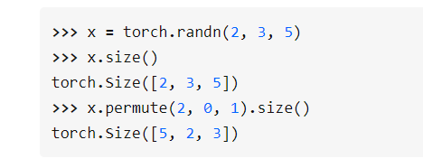
torch.Tensor.permute(dims)

作用：将tensor的纬度换位。
参数：
dims：换位顺序
举例：

参考链接

FLOWVERSE

关注

10
点赞
踩
36

收藏

觉得还不错? 一键收藏
打赏
8
评论
GC-Net 笔记及探讨 --- unary特征以及级联的cost volume （更新中）

前言之前读AANet，读patchmatch-net，读pam-net，读各种fancy的net的时候，总是会不停的往前追溯，总会追溯到GC-net，借鉴到GC-net的思想。因此，决定精读GC-Net，并做以下笔记。论文结构近几年总说的cost volume，其实就来源于这篇GC-Net。在看网络结构之前，先看看看论文结构吧。IntroductionRelated WorkLearning End-to-end Disparity Regression3.1 Unary Features
复制链接

扫一扫