【理论推导】随机微分方程(SDE)视角下的Diffusion Model与Score-based Model

SDE与DDPM

以 DDPM 为例，DDPM的通项公式为
$$x_t\sim \mathcal{N}(\sqrt{{\overline{\alpha }}_t}{x}_0,(1-{\overline{\alpha }}_t)I)$$
当我们固定 $t$ 的取值时，$x_t$ 是定义在样本空间上的函数，即为一随机变量，当我们固定$x$的随机性时，即为关于变量 $t$ 的一个函数，因此 $x_t$ 是一随机过程，而对于一组确定的 { x t } t = 0 T \{x_t\}_{t=0}^T {xt​}t=0T​，称为随机过程的一个实现，或是一条轨迹/轨道，而随机过程可以使用随机微分方程(Stochastic Differential Equation)进行描述

SDE定义为
$$d{X}_t=b(t,X_t)dt+\sigma (t,X_t)d{B}_t$$
其中 $B_t$ 表示布朗运动，此方程的解称为伊藤(Itô)过程或是扩散过程。如果我们将 DDPM的迭代式从离散扩展到连续区间，即 $x_t\to x_{t+\Delta t}(\Delta t\to 0)$，即可得到SDE形式的扩散过程，论文中表示为
$$dx=f(x,t)dt+g(t)dw$$
其中 $w$ 表示一个标准布朗运动，$f(\cdot ,t)$ 称作是漂移系数 (drift coefficient)，描述了确定性的变化过程，$g(\cdot )$ 称作是扩散系数 (diffusion coefficient)，描述了不确定的变化过程

SDE视角下的生成模型

SDE的离散形式表示如下所示
$$x_{t+{\Delta }_t}-x_t=f(x,t)\Delta t+g(t)\sqrt{\Delta t}\epsilon$$
其中 $\epsilon \sim \mathcal{N}(0,I)$，因此有条件概率分布
$$x_{t+{\Delta }_t}|x_t\sim \mathcal{N}(x_t+f(x_t,t)\Delta t,g^2(t)\Delta tI)$$
考虑逆过程 $x_t|x_{t+\Delta t}$，有
p ( x t ∣ x t + Δ t ) = p ( x t + Δ t ∣ x t ) p ( x t ) p ( x t + Δ t ) = p ( x t + Δ t ∣ x t ) exp ⁡ ( log ⁡ p ( x t ) − log ⁡ p ( x t + Δ t ) ) ≈ p ( x t + Δ t ∣ x t ) exp ⁡ { − ( x t + Δ t − x t ) ▽ x t log ⁡ p ( x t ) − Δ t ∂ ∂ t log ⁡ p ( x t ) } ∝ exp ⁡ { − ∣ ∣ x t + Δ t − x t − f ( x t , t ) Δ t ∣ ∣ 2 2 2 g 2 ( t ) Δ t − ( x t + Δ t − x t ) ▽ x t log ⁡ p ( x t ) − Δ t ∂ ∂ t log ⁡ p ( x t ) } = exp ⁡ { − 1 2 g 2 ( t ) Δ t ∣ ∣ ( x t + Δ t − x t ) − ( f ( x t , t ) − g 2 ( t ) ▽ x t log ⁡ p ( x t ) ) Δ t ∣ ∣ 2 2 − Δ t ∂ ∂ t log ⁡ p ( x t ) − f 2 ( x t , t ) Δ t 2 g 2 ( t ) + ( f ( x t , t ) − g 2 ( t ) ▽ x t log ⁡ p ( x t ) ) 2 Δ t 2 g 2 ( t ) } = Δ t → 0 exp ⁡ { − 1 2 g 2 ( t + Δ t ) Δ t ∣ ∣ ( x t + Δ t − x t ) − ( f ( x t + Δ t , t + Δ t ) − g 2 ( t + Δ t ) ▽ x t + Δ t log ⁡ p ( x t + Δ t ) ) Δ t ∣ ∣ 2 2 } \begin{align} p(x_t|x_{t+\Delta t}) &= \frac{p(x_{t+\Delta t}|x_t)p(x_t)}{p(x_{t+\Delta t})} \nonumber \\&= p(x_{t+\Delta t}|x_t)\exp(\log p(x_t)-\log p(x_{t+\Delta t})) \nonumber \\&\approx p(x_{t+\Delta t}|x_t)\exp \{ - (x_{t+\Delta t}-x_t)\triangledown_{x_t} \log p(x_t)-\Delta t \frac{\partial }{\partial t}\log p(x_{t})\} \nonumber \\&\propto \exp \{-\frac{||x_{t+\Delta t}-x_t - f(x_t,t)\Delta t||_2^2}{2g^2(t)\Delta t} - (x_{t+\Delta t} - x_t)\triangledown_{x_t}\log p(x_t)- \Delta t \frac{\partial }{\partial t}\log p(x_t)\} \nonumber \\&= \exp \left\{ -\frac{1}{2g^2(t)\Delta t}||(x_{t+\Delta t}-x_t)-(f(x_t,t)-g^2(t)\triangledown_{x_t}\log p(x_t))\Delta t||_2^2 -\Delta t \frac{\partial }{\partial t}\log p(x_t) - \frac{f^2(x_t,t)\Delta t}{2g^2(t)} + \frac{(f(x_t,t)-g^2(t)\triangledown_{x_t}\log p(x_t))^2\Delta t}{2g^2(t)} \right\} \nonumber \\&\overset{\Delta t\rightarrow 0}{=} \exp \left\{ -\frac{1}{2g^2(t+\Delta t)\Delta t}||(x_{t+\Delta t}-x_t)-(f(x_{t+\Delta t},t+\Delta t)-g^2(t+\Delta t)\triangledown_{x_{t+\Delta t}}\log p(x_{t+\Delta t}))\Delta t||_2^2 \right \} \nonumber \end{align} p(xt​∣xt+Δt​)​=p(xt+Δt​)p(xt+Δt​∣xt​)p(xt​)​=p(xt+Δt​∣xt​)exp(logp(xt​)−logp(xt+Δt​))≈p(xt+Δt​∣xt​)exp{−(xt+Δt​−xt​)▽xt​​logp(xt​)−Δt∂t∂​logp(xt​)}∝exp{−2g2(t)Δt∣∣xt+Δt​−xt​−f(xt​,t)Δt∣∣22​​−(xt+Δt​−xt​)▽xt​​logp(xt​)−Δt∂t∂​logp(xt​)}=exp{−2g2(t)Δt1​∣∣(xt+Δt​−xt​)−(f(xt​,t)−g2(t)▽xt​​logp(xt​))Δt∣∣22​−Δt∂t∂​logp(xt​)−2g2(t)f2(xt​,t)Δt​+2g2(t)(f(xt​,t)−g2(t)▽xt​​logp(xt​))2Δt​}=Δt→0exp{−2g2(t+Δt)Δt1​∣∣(xt+Δt​−xt​)−(f(xt+Δt​,t+Δt)−g2(t+Δt)▽xt+Δt​​logp(xt+Δt​))Δt∣∣22​}​

因此，$x_t|x_{t+\Delta t}$ 服从均值方差如下的高斯分布
$$\begin{gathered} \mu =x_{t+\Delta t}-(f(x_{t+\Delta t},t+\Delta t)-g^2(t+\Delta t){▽}_{x_{t+\Delta t}}\log p(x_{t+\Delta t}))\Delta t \\ {\sigma }^2=g^2(t+\Delta t)\Delta t \end{gathered}$$
因此，有SDE表示逆过程离散形式与连续形式如下所示
$$\begin{array}{rl}{x}_{t+\Delta t}-x_t& =(f(x_{t+\Delta t},t+\Delta t)-g^2(t+\Delta t){▽}_{x_{t+\Delta t}}\log p(x_{t+\Delta t}))\Delta t+g(t+\Delta t)\sqrt{\Delta t}\epsilon \\ dx& =[f(x,t)-g^2(t){▽}_{x_t}\log p(x_t)]+g(t)dw\end{array}$$

考虑 NCSN 与 DDPM，两种形式均可以统一到SDE的理论表示形式下面，分别称为 VE-SDE (Variance Exploding) 与 VP-SDE (Variance Preserving)，对应 NCSN 与 DDPM

对于NCSN，正向过程（加噪声）如下所示
$$\begin{gathered} x_t=x_0+{\sigma }_t\epsilon \\ {x}_{t+1}=x_t+\sqrt{{\sigma }_{t+1}^2-{\sigma }_t^2}\epsilon \end{gathered}$$
因此，对应的SDE表示形式中
$$\begin{gathered} f(x_t,t)=0 \\ g(t)=\frac{d}{dt}{\sigma }_t^2 \end{gathered}$$

对于 DDPM，正向过程（加噪声）如下所示
$$\begin{gathered} x_t=\sqrt{{\overline{\alpha }}_t}{x}_0+\sqrt{1-{\overline{\alpha }}_t}\epsilon \\ {x}_{t+1}=\sqrt{1-{\beta }_{t+1}}{x}_t+\sqrt{{\beta }_{t+1}}\epsilon \end{gathered}$$
我们令 $\beta :[0,1]\to \mathbb{R}$ 代替 ${\beta }_t$，满足 $\beta (\frac{i}{T})=T{\beta }_i$，$\Delta t=\frac{1}{T}$，则有
$$\begin{array}{rl}{x}_{t+1}& =\sqrt{1-\beta (t+\Delta t)\Delta t}{x}_t+\sqrt{\beta (t+\Delta t)\Delta t}\epsilon \\ & \stackrel{\Delta t\to 0}{=}(1-\frac{1}{2}\beta (t)\Delta t)x_t+\sqrt{\beta (t)}\sqrt{\Delta t}\epsilon \end{array}$$
因此，对应的SDE表现形式中，有
$$\begin{gathered} f(x_t,t)=-\frac{1}{2}\beta (t)x_t \\ g(t)=\sqrt{\beta (t)} \end{gathered}$$

当我们希望 $t\to T$ 时，图像为纯粹的噪声图像，那么 ${\sigma }_t\to \infty$，但 ${\overline{\alpha }}_t\to 0$ 即可，因此分别称作是 VE-SDE 和 VP-SDE

DDPM Denoiser ${ϵ}_{\theta }(x_t,t)$ 与 NCSN Estimator $s_{\theta }(x_t,t)$ ：在 DDPM 正向过程中，有 $x_t\sim \mathcal{N}({\sqrt{\overline{\alpha }}}_t{x}_0,(1-{\overline{\alpha }}_t)I)$，代入 $s_{\theta }(x_t,t)={▽}_{x_t}\log p(x_t)$，可以得到
$$s_{\theta }(x_t,t)=-\frac{x_t-{\sqrt{\overline{\alpha }}}_t{x}_0}{1-{\overline{\alpha }}_t}=-\frac{1}{\sqrt{1-{\overline{\alpha }}_t}}{ϵ}_{\theta }(x_t,t)$$

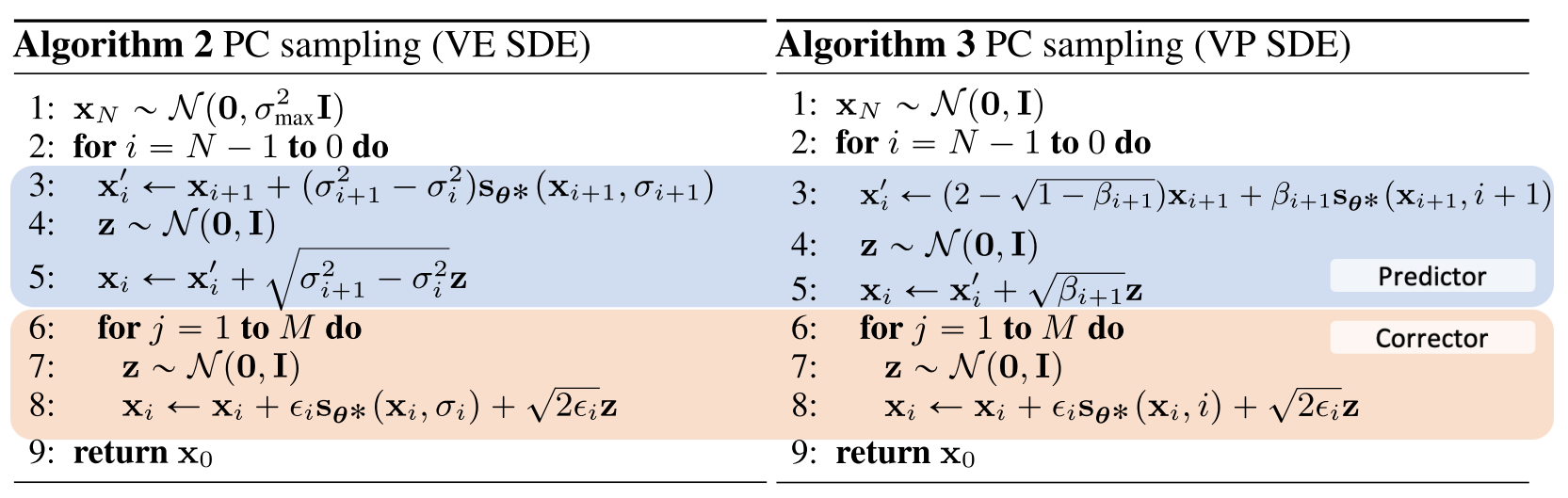
PC Sampling

最后，从算法实现的角度来回顾一下 DDPM 和 NCSN，DDPM基于的假设是 Markov 假设，假定不同时间的采样之间服从条件概率分布，因此 DDPM 采用称作是祖先采样(Ancestral Sampling)的方式去求解 SDE 方程，给出的算法如下所示

而 NCSN 依赖于 Langevin Dynamics 进行同一噪声分布下的迭代优化，对于不同的噪声大小，得到的采样之间并没有进行任何的依赖关系，其采样方式如下所示

前者可以看作是对于 SDE 方程的离散形式求解，称为Predictor，后者可以看作是进一步的优化过程，称为 Corrector，作者结合这两部分，给出了 Predictor-Corrector Sampling Method

参考资料

Score-based Generative Modeling Through Stochastic Differential Equations

扩散模型 Diffusion Model SDE