Lime 代码

import lime
from lime import lime_image

explainer = lime_image.LimeImageExplainer()
explanation = explainer.explain_instance(image, classifier_fn, labels=(1,),
                         hide_color=None,
                         top_labels=5, num_features=100000, num_samples=1000,
                         batch_size=10,
                         segmentation_fn=None,
                         distance_metric='cosine',
                         model_regressor=None,
                         random_seed=None)

参数说明：

image:待解释图像

classifier_fn:分类器

labels:可解析标签

hide_color:隐藏颜色

top_labels:预测概率最高的K个标签生成解释

num_features:说明中出现的最大功能数

num_samples:学习线性模型的邻域大小

batch_size:批处理大小

distance_metric:距离度量

model_regressor:模型回归器，默认为岭回归

segmentation_fn:分段，将图像分为多个大小

random_seed:随机整数，用作分割算法的随机种子

具体实现过程如下，我用lime查看我自己训练的efficientB1模型，具体代码如下：

"""
可解释模型算法
"""
import lime
from lime import lime_image
import numpy as np
from keras.preprocessing import image
import matplotlib.pyplot as plt
from skimage.segmentation import mark_boundaries
import PIL.Image as Image
from keras.applications.densenet import preprocess_input
from keras.models import load_model
from nets import efficientnet


def transform_img_fn(img_name,model):
    out = []
    img = image.load_img(img_name,target_size=(240,240))
    x = image.img_to_array(img)
    x = np.expand_dims(x,axis=0)
    x = preprocess_input(x)
    #out.append(x)
    #return np.vstack(out)
    return x

if __name__ == '__main__':
    img_name = r"15_sr.png"
    model_predict_01 = load_model("EfficientNetB1.model")       #加载模型
    images = transform_img_fn(img_name,model_predict_01)
    explainer = lime_image.LimeImageExplainer()
    x = images[0].astype(np.double)
    explanation = explainer.explain_instance(x,model_predict_01.predict,top_labels=5,hide_color=0,num_samples=1000)
    print(explanation)
    #对图像分类结果进行解释
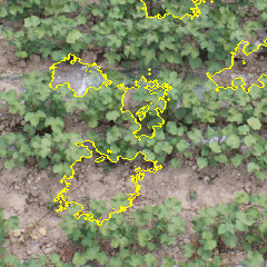
    temp,mask = explanation.get_image_and_mask(explanation.top_labels[0],positive_only=True, negative_only=False,num_features=5,hide_rest=False)
    img = io.imread(img_name)
    img = transform.resize(img, (240,240))
    image = img_as_float(img)
    plt.imsave("out.jpg",mark_boundaries(image,mask))

解析的结果如下：