智能优化算法（源码）-食肉植物算法（Carnivorous Plant Algorithm ，CPA)

获取更多资讯，赶快关注上面的公众号吧！

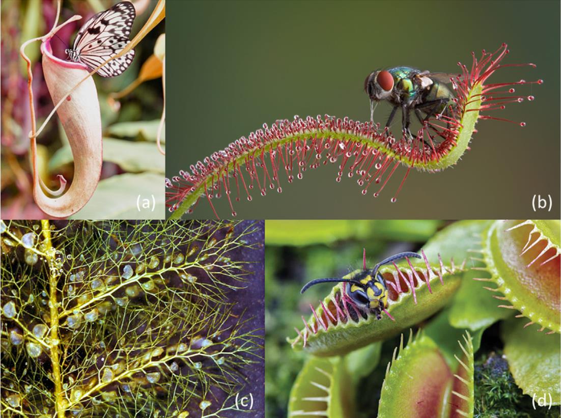
  食肉植物算法 carnivorous plant algorithm (CPA)是由马拉西亚的Ong Kok Meng，于2020年受食肉植物如何适应恶劣环境（比如捕食昆虫和传粉繁殖）的启发而提出的。扫码关注公众号，后台回复“食肉植物”或“CPA”可以获取Matlab代码。

背景

  众所周知，大多数植物是动物的直接食物来源，但是自然界中也有例外，食肉植物就是其中一种。它们通常生长在缺乏营养的恶劣环境中，例如，湿地、沼泽和以水丰富为特征的泥泞海岸。为了获取生长和繁殖所需的氮和磷等额外的营养，食肉植物用它们分泌的酶吸引、诱捕和吃掉苍蝇、蝴蝶、蜥蜴和老鼠等动物。猪笼草、茅膏菜、狸藻、维纳斯捕蝇草等都是常见的食肉植物。[PS:北航还在猪笼草身上发现了水倒流的现象，并因此成功发表了全国机械领域的第一篇Nature]

图1 常见的食肉植物

食肉植物算法的数学模型

  那么接下来就介绍一下用于模拟食肉植物吸引、诱捕、消化和繁殖策略的数学模型。CPA从随机初始化一组解开始，然后这些解被分为食肉植物和猎物，再按生长和繁殖过程分组，进行适应度值的更新，最后将所有解合并。整个过程循环执行直到满足终止条件。

初始化

  CPA是一种基于种群的优化算法，因此首先需要初始化待求解问题的可能解，即在湿地中随机初始化$nCPlant$个食肉植物和$nPrey$个猎物个体，每个个体的位置由以下矩阵表示：
$$Pop=\left[\begin{array}{ccccc}{\text{ Individual }}_{1,1}& {\text{ Individual }}_{1,2}& \cdots & \cdots & {\text{ Individual }}_{1,d}\\ {\text{ Individual }}_{2,1}& {\text{ Individual }}_{2,2}& \cdots & \cdots & {\text{ Individual }}_{2,d}\\ ⋮& ⋮& ⋮& ⋮& ⋮\\ ⋮& ⋮& ⋮& ⋮& ⋮\\ {\text{ Individual }}_{n,1}& {\text{ Individual }}_{n,2}& \cdots & \cdots & {\text{ Individual }}_{n,d}\end{array}\right]\text{\hspace{1em}(1)}$$
其中$d$为维度，即变量个数，$n$为$nCPlant$和$nPrey$的总和，每个个体使用下式进行随机初始化：
$${\text{ Individual }}_{i,j}=L{b}_j+\left(U{b}_j-L{b}_j\right)\times \text{ rand }\text{\hspace{1em}(2)}$$
其中，$Lb$和$Ub$分别为搜索域的下界和上界，即自变量的最小值和最大值，$i\in [1,2,...,n]$,$j\in [1,2,...,d]$,$rand$为$[0,1]$之间的随机数。

  对于第$i$个个体，通过将每一行（即所有维度）作为适应度函数的输入来评估适应度值，计算得到的适应度值存储在以下矩阵中：
$$\text{ Fit }=\left[\begin{array}{ccccc}f({\text{ Individual }}_{1,1}& {\text{ Individual }}_{1,2}& \cdots & \cdots & \text{ Individual }{}_{1,d})\\ f({\text{ Individual }}_{2,1}& {\text{ Individual }}_{2,2}& \cdots & \cdots & \text{ Individual }{}_{2,d})\\ & ⋮& & & \\ & ⋮& & & \\ f({\text{ Individual }}_{n,1}& {\text{ Individual }}_{n,2}& \cdots & \cdots & \text{ Individual }{}_{n,d})\end{array}\right]\text{\hspace{1em}(3)}$$

分类和分组

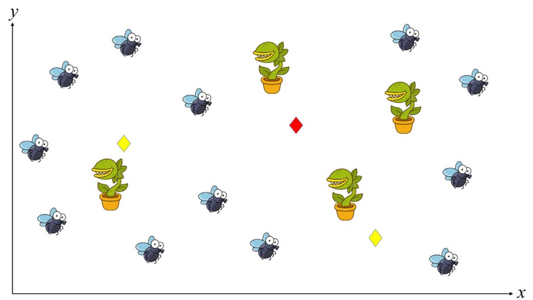
  接下来，式（1）中的每个个体按照其适应度值升序排序（考虑最小化问题），那么排在最前面的$nCPlant$个解就作为食肉植物$CP$，而剩余的$nPrey$个解就是猎物$Prey$。图2可视化了食肉植物和猎物种群。

图2 食肉植物和猎物种群，其中红色钻石表示全局最优解，黄色钻石表示局部最优解

  排序后的适应度值和种群可通过式（4）和式（5）表达：

$$\text{ Sorted\_Fit }=\left[\begin{array}{c}{f}_{CP(1)}\\ f_{CP(2)}\\ ⋮\\ f_{CP(nCPlant)}\\ f_{\text{Prey }(nCPlant+1)}\\ f_{\text{Prey }(nCPlant+2)}\\ ⋮\\ f_{\text{Prey }(nCPlant+nprey)}\end{array}\right]\text{\hspace{1em}(4)}$$

Sorted_Pop
$$=\left[\begin{array}{ccccc}C{P}_{1,1}& C{P}_{1,2}& \cdots & \cdots & C{P}_{1,d}\\ C{P}_{2,1}& C{P}_{2,2}& \cdots & \cdots & C{P}_{2,d}\\ ⋮& ⋮& ⋮& ⋮& ⋮\\ C{P}_{nCPlant},1& C{P}_{nCPlant,2}& \cdots & \cdots & C{P}_{nCPlant,d}\\ {\text{ Prey }}_{nCPlant+1,1}& {\text{ Prey }}_{nCPlant+1,2}& \cdots & \cdots & {\text{ Prey }}_{nCPlant+1,d}\\ {\text{ Prey }}_{nCPlant+2,1}& {\text{ Prey }}_{nCPlant+2,2}& \cdots & \cdots & {\text{ Prey }}_{nCPlant+2,d}\\ ⋮& ⋮& ⋮& ⋮& ⋮\\ {\text{ Prey }}_{nCPlant+nPrey,1}& {\text{ Prey }}_{nCPlant+nPrey,2}& \cdots & \cdots & {\text{ Prey }}_{nCPlant+nPrey,d}\end{array}\right]\text{\hspace{1em}(5)}$$

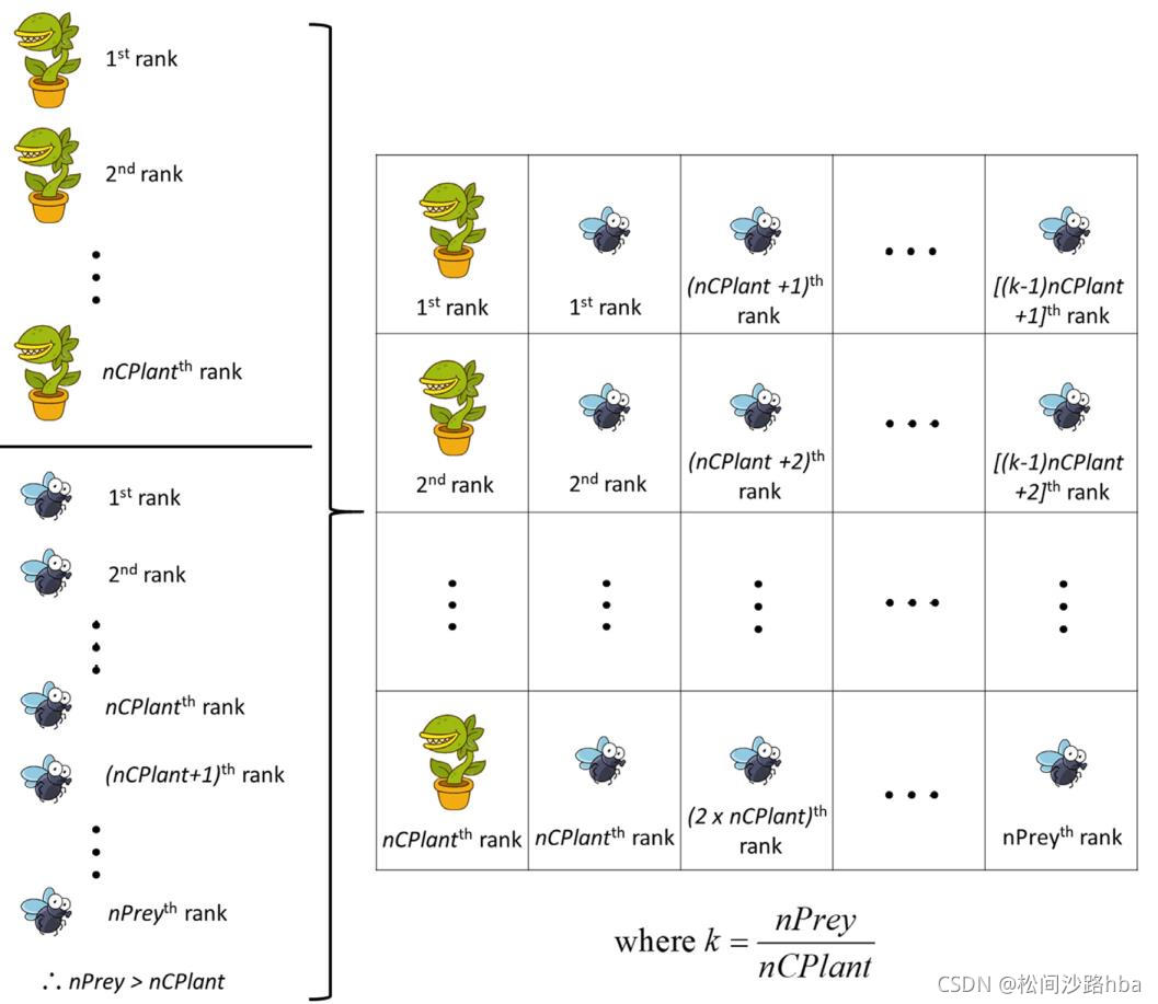
  分组的过程主要是用于模拟每个食肉植物及其猎物的环境，在分组过程中，将适合度值最高的猎物分配给排名第一的食肉植物，类似地，第二名和第三名猎物分别属于第二和第三名食肉植物。重复该过程，直到排名第$nCPlant$的猎物分配给排名第$nCPlant$的食肉植物，然后第$nCPlant+1$名猎物分配给第1名食肉植物（所以这里默认猎物是多余食肉植物的）。整个分组过程入图3所示。对食肉植物进行分组主要是为了减少食肉植物生长过程中出现大量劣质猎物的可能性，这对提高食肉植物的生存能力至关重要。

图3 CPA的分组过程

成长（探索）

  由于土壤营养不良，食肉植物会吸引、诱捕和消化猎物来生长。这种植物的香味能引诱猎物，但猎物也能偶尔成功地从食肉植物的魔爪中逃脱，所以这里引入了一个吸引率。

  每一种群都随机选择一个猎物，如果吸引率高于随机生成的数字，食肉植物就会捕获猎物并消化来生长。新的食肉植物的生长模型为：
$${\text{ NewCP }}_{i,j}=\text{ growth }\times C{P}_{i,j}+(1-\text{ growth })\times {\text{ Prey }}_{v,j}\text{\hspace{1em}(6)}$$

$$\text{ growth }=growth\_rate\times {\text{ rand }}_{i,j}\text{\hspace{1em}(7)}$$

其中$C{P}_{i,j}$是排名第$i$的食肉植物，$Pre{y}_{v,j}$为随机选择的猎物，成长率$growth\_rate$为预定义的值，$rand$为$[0,1]$之间的随机数。在CPA中，每一个种群内部只有一个食肉植物，而猎物的数量必须多于两个。大多数情况下，CPA的吸引率设置为0.8。

  另一方面，如果吸引率低于产生的随机值，则猎物设法逃脱陷阱并继续生长，数学上表示为:

$${\text{ NewPrey }}_{i,j}=\text{ growth }\times {\text{ Prey }}_{u,j}+(1-\text{ growth })\times {\text{ Prey }}_{v,j},u\ne v\text{\hspace{1em}(8)}$$

$$f(n)=\{\begin{array}{ll}\text{ growth\_rate }\times {\text{ rand }}_{i,j},& f\left({\text{ prey }}_v\right)>f\left({\text{ prey }}_u\right)\\ 1-\text{ growth\_rate }\times {\text{ rand }}_{i,j},& f\left({\text{ prey }}_v\right)<f\left({\text{ prey }}_u\right)\end{array}\text{\hspace{1em}(9)}$$

其中$Pre{y}_{u,j}$是第$i$个种群中随机选择的另一个猎物。食肉植物和猎物的生产过程都将持续$\text{group\_iter}$代。

  式（6）和（8)用于将新的解向高质量解空间方向指引，同时也为了保证在猎物的生长过程中起到类似的作用，引入了式（9），因为随机选择的$Pre{y}_u$可能劣于$Pre{y}_v$。如式（6）和（8）所示，算法的探索受生长率的影响，生长率越高，探索范围越大，错失全局最优解的可能性业越大。因此需要选择一个合适的生长率。

繁殖（利用）

  食肉植物吸收猎物的营养，并利用这些营养生长和繁殖。在繁殖方面，只有排名第一的食肉植物，即种群中最好的解，才允许繁殖。这是为了确保CPA的利用只关注最优解，从而避免对其他解进行不必要的利用，节省计算成本。最优食肉植物的繁殖过程如下：
$${\text{ NewCP }}_{i,j}=C{P}_{1,j}+\text{ Reproduction\_rate }\times {\text{ rand }}_{i,j}\times {\text{ mate }}_{i,j}\text{\hspace{1em}(10)}$$

$${\text{ mate }}_{i,j}=\{\begin{array}{ll}C{P}_{v,j}-C{P}_{i,j}& f\left(C{P}_i\right)>f\left(C{P}_v\right)\\ C{P}_{i,j}-C{P}_{v,j}& f\left(C{P}_i\right)<f\left(C{P}_v\right)\end{array},i\ne v\ne 1\text{\hspace{1em}(11)}$$

其中$C{P}_{1,j}$为最优解，$C{P}_{v,j}$为随机选择的食肉植物，繁殖率$Reproduction\_rate$是预定义的用于利用的值。繁殖过程重复$nCPlant$次，繁殖过程中，为每个维度$j$都随机选择一个食肉植物$v$。

适应度更新和合并

  将新生成的食肉植物和猎物于先前的种群进行合并，就得到了一个新的维度为$[n+nCPlant(group\_iter+nCPlant)]\text{x}d$维（$n$个原始个体，$nCPlant(group\_iter$个生长过程个体和$nCPlant$个繁殖过程个体）的新种群，之后，新种群按照适应度值升序排序，选择排名前$n$的个体作为新的候选解，保证种群大小不变。这种精英选择策略保证了选择更优的解用于下一代的繁殖。

停止准则

  重复整个分类、分组、生长和繁殖的过程，直到到达终止停止准则。如下 为CPA的伪代码。

食肉植物算法

1.定义目标函数$f(\vec{x}),\vec{x}=\left(x_1,x_2,..,x_d\right)$

2.定义组内迭代次数$group\_iter$、吸引率$attraction\_rate$、生长率$growth\_rate$、繁殖率$reproduction\_rate$、食肉植物数量$nCPlant$和猎物数量$nPrey$

3.随机初始化大小为$n$、维度为$d$的种群

4.评估每个个体的适应度值

5.找到最优个体$g^{\ast }$作为排名第一的食肉植物

6.Repeat until 满足终止条件

7. 将排名前$nCPlant$的个体分类为食肉植物

8. 将剩余的$nPrey$个个体分类为猎物

9. 将食肉植物和猎物进行分组

10. // 食肉食物和猎物的生长过程

11. for $i=1:nCPlant$

12.  for $Group\_cycle=1:group\_iter$

13.   if $attraction\_rate>随机数$

14.    根据式（6）生成新的食肉植物

15.   else

16.    根据式（8）生成新的猎物

17.  end for

18. end for

19. //最优食肉植物的繁殖过程

20. for $i=1:nCPlant$

21.  根据式（10）基于最优食肉植物生成新的食肉植物

22. end for

23. 评估新生成的每个食肉植物和猎物

24. 合并之前和新生成的食肉植物和猎物

25. 对个体进行排序，并选择前$n$个个体进入下一代

26. 确定当前最优个体$g^{\ast }$作为排名第一的食肉植物

27.end while

28.展示当前最优解$g^{\ast }$