Chatglm2-6b模型解析

hjyai94

已于 2023-11-21 18:23:29 修改

阅读量2.7k

点赞数 1

文章标签： chatgpt 人工智能 nlp transformer

于 2023-08-25 23:03:34 首次发布

本文链接：https://blog.csdn.net/hjyai94/article/details/132504200

版权

本文利用chatglm2-6b huggingface上的模型源码介绍其结构，结合一些论文博客对chatglm2模型进行分解。

模型参数

Chatglm2-6b模型参数包括28个GLM层（由MLP和自注意力组成），注意力的头数为32，采用Multi-Query Attention，隐藏层层数28。位置编码采用旋转位置编码，激活函数为SwiGLU，归一化方法为RMSNorm。

整体模型结构

ChatGLMModel (假设输入X大小为 3x5)

(embedding) Embedding (转置后 5x3x4096)
- word_embeddings: Embedding(65024, 4096)
(rotary_pos_emb) RotaryEmbedding()
(encoder) GLMTransformer
- (layers) ModuleList
  - 0-27: 28 x GLMBlock
    - (input_layernorm) RMSNorm() (输入输出大小: 5x3x4096)
    - (self_attention) SelfAttention
      - (query_key_value) Linear(in_features=4096, out_features=4608, bias=True)
      - (core_attention) CoreAttention(
        (attention_dropout) Dropout(p=0.0, inplace=False))
      - (dense) Linear(in_features=4096, out_features=4096, bias=False)
    - (post_attention_layernorm) RMSNorm()
    - (mlp) MLP
      - (dense_h_to_4h) Linear(in_features=4096, out_features=27392, bias=False)
      - (dense_4h_to_h) Linear(in_features=13696, out_features=4096, bias=False)
- (final_layernorm) RMSNorm()
(output_layer) Linear(in_features=4096, out_features=65024, bias=False) (输出大小: 3x5x65024)

激活函数：SwiGLU

$\operatorname{SwiGLU(x, W, V, b, c, \beta)}=\operatorname{Swish}_{\beta}(x W+b) \otimes(xV+c)$
其中 $\operatorname{Swish}_\beta(x)=x \sigma(\beta x)$ , $\beta$ 为指定常数，常为1。
对应于chatglm2-6b中的源码

def swiglu(x):
    x = torch.chunk(x, 2, dim=-1)
    return F.silu(x[0]) * x[1]

旋转位置编码：RoPE
旋转位置编码的目的是用上不同token的相对位置。
假定 query 向量 $\boldsymbol{q}_m$ 和 key 向量 $\boldsymbol{k}_n$ 之间的内积操作可以被一个函数 $g$ 表示，该函数 $g$ 的输入是词嵌入向量 $\boldsymbol{x}_m ， \boldsymbol{x}_n$ 和它们之间的相对位置为 $m - n$ :
$\left\langle\boldsymbol{f}_q\left(\boldsymbol{x}_m, m\right), f_k\left(\boldsymbol{x}_n, n\right)\right\rangle=g\left(\boldsymbol{x}_m, \boldsymbol{x}_n, m-n\right)$
这样就能够将原来的绝对位置编码转为相对位置编码，下面就是求解 $g$ 就可以了。苏剑林等人的论文中提出了如下的公式解决该问题。具体推导过程也可以参考该作者的博客。
$\begin{aligned} & f_q\left(\boldsymbol{x}_m, m\right)=\left(\boldsymbol{W}_q \boldsymbol{x}_m\right) e^{i m \theta} \\ & \quad f_k\left(\boldsymbol{x}_n, n\right)=\left(\boldsymbol{W}_k \boldsymbol{x}_n\right) e^{i n \theta} \\ & g\left(\boldsymbol{x}_m, \boldsymbol{x}_n, m-n\right)=\operatorname{Re}\left[\left(\boldsymbol{W}_q \boldsymbol{x}_m\right)\left(\boldsymbol{W}_k \boldsymbol{x}_n\right)^* e^{i(m-n) \theta}\right]\end{aligned}$
进一步地， $f_q$ 可以表示成下面的式子:
$\begin{aligned} f_q\left(\boldsymbol{x}_m, m\right) & =\left(\begin{array}{cc}\cos m \theta & -\sin m \theta) \\ \sin m \theta & \cos m \theta\end{array}\right)\left(\begin{array}{ll}W_q^{(1,1)} & W_q^{(1,2)} \\ W_q^{(2,1)} & W_q^{(2,2)}\end{array}\right)\left(\begin{array}{c}x_m^{(1)} \\ x_m^{(2)}\end{array}\right) \\ & =\left(\begin{array}{cc}\cos m \theta & -\sin m \theta) \\ \sin m \theta & \cos m \theta\end{array}\right)\left(\begin{array}{c}q_m^{(1)} \\ q_m^{(2)}\end{array}\right)\end{aligned}$
看到这里会发现，这不就是 query 向量乘以了一个旋转矩阵吗? 这就是为什么叫做旋转位置编码的原因。
同理， $f_k$ 可以表示成下面的式子:
$\begin{aligned} f_k\left(\boldsymbol{x}_m, m\right) & =\left(\begin{array}{cc}\cos m \theta & -\sin m \theta) \\ \sin m \theta & \cos m \theta\end{array}\right)\left(\begin{array}{ll}W_k^{(1,1)} & W_k^{(1,2)} \\ W_k^{(2,1)} & W_k^{(2,2)}\end{array}\right)\left(\begin{array}{c}x_m^{(1)} \\ x_m^{(2)}\end{array}\right) \\ & =\left(\begin{array}{cc}\cos m \theta & -\sin m \theta) \\ \sin m \theta & \cos m \theta\end{array}\right)\left(\begin{array}{l}k_m^{(1)} \\ k_m^{(2)}\end{array}\right)\end{aligned}$
最终 $g\left(\boldsymbol{x}_m, \boldsymbol{x}_n, m-n\right)$ 可以表示如下:
$g\left(\boldsymbol{x}_m, \boldsymbol{x}_n, m-n\right)=\left(\begin{array}{ll}\boldsymbol{q}_m^{(1)} & \boldsymbol{q}_m^{(2)}\end{array}\right)\left(\begin{array}{cc}\cos ((m-n) \theta) & -\sin ((m-n) \theta) \\ \sin ((m-n) \theta) & \cos ((m-n) \theta)\end{array}\right)\left(\begin{array}{c}k_n^{(1)} \\ k_n^{(2)}\end{array}\right)$
将上面的式子扩展到任意维度，可以表示如下：
$f_{\{q, k\}}\left(\boldsymbol{x}_m, m\right)=\boldsymbol{R}_{\Theta, m}^d \boldsymbol{W}_{\{q, k\}} \boldsymbol{x}_m$
因为内积具有线性累加性，所以任意偶数维的RoPE，都可以表示为二维情形的拼接，即
$\boldsymbol{R}_{\Theta, m}^d=\left(\begin{array}{ccccccc}\cos m \theta_1 & -\sin m \theta_1 & 0 & 0 & \cdots & 0 & 0 \\ \sin m \theta_1 & \cos m \theta_1 & 0 & 0 & \cdots & 0 & 0 \\ 0 & 0 & \cos m \theta_2 & -\sin m \theta_2 & \cdots & 0 & 0 \\ 0 & 0 & \sin m \theta_2 & \cos m \theta_2 & \cdots & 0 & 0 \\ \vdots & \vdots & \vdots & \vdots & \ddots & \vdots & \vdots \\ 0 & 0 & 0 & 0 & \cdots & \cos m \theta_{d / 2} & -\sin m \theta_{d / 2} \\ 0 & 0 & 0 & 0 & \cdots & \sin m \theta_{d / 2} & \cos m \theta_{d / 2}\end{array}\right)$
考虑到上述矩阵的稀疏性，利用矩阵计算会十分浪费算力，因此推荐使用如下的方式实现：
$\boldsymbol{R}_{\Theta, m}^d \boldsymbol{x}=\left(\begin{array}{c}x_0 \\ x_1 \\ x_2 \\ x_3 \\ \vdots \\ x_{d-2} \\ x_{d-1}\end{array}\right) \otimes\left(\begin{array}{c}\cos m \theta_0 \\ \cos m \theta_0 \\ \cos m \theta_1 \\ \cos m \theta_1 \\ \vdots \\ \cos m \theta_{d / 2-1} \\ \cos m \theta_{d / 2-1}\end{array}\right)+\left(\begin{array}{c}-x_1 \\ x_0 \\ -x_3 \\ x_2 \\ \vdots \\ -x_{d-1} \\ x_{d-2}\end{array}\right) \otimes\left(\begin{array}{c}\sin m \theta_0 \\ \sin m \theta_0 \\ \sin m \theta_1 \\ \sin m \theta_1 \\ \vdots \\ \sin m \theta_{d / 2-1} \\ \sin m \theta_{d / 2-1}\end{array}\right)$
其中， $\otimes$ 表示按位相乘对应于pytorch中的*运算。
chatglm2-6b中的代码实现：

class RotaryEmbedding(nn.Module):
    def __init__(self, dim, original_impl=False, device=None, dtype=None):
        super().__init__()
        inv_freq = 1.0 / (10000 ** (torch.arange(0, dim, 2, device=device).to(dtype=dtype) / dim))
        self.register_buffer("inv_freq", inv_freq)
        self.dim = dim
        self.original_impl = original_impl

    def forward_impl(
            self, seq_len: int, n_elem: int, dtype: torch.dtype, device: torch.device, base: int = 10000
    ):
        """Enhanced Transformer with Rotary Position Embedding.

        Derived from: https://github.com/labmlai/annotated_deep_learning_paper_implementations/blob/master/labml_nn/
        transformers/rope/__init__.py. MIT License:
        https://github.com/labmlai/annotated_deep_learning_paper_implementations/blob/master/license.
        """
        # $\Theta = {\theta_i = 10000^{\frac{2(i-1)}{d}}, i \in [1, 2, ..., \frac{d}{2}]}$
        theta = 1.0 / (base ** (torch.arange(0, n_elem, 2, dtype=dtype, device=device) / n_elem))

        # Create position indexes `[0, 1, ..., seq_len - 1]`
        seq_idx = torch.arange(seq_len, dtype=dtype, device=device)
        # Calculate the product of position index and $\theta_i$
        idx_theta = torch.outer(seq_idx, theta).float()
        cache = torch.stack([torch.cos(idx_theta), torch.sin(idx_theta)], dim=-1)
        return cache

    def forward(self, max_seq_len, offset=0):
        return self.forward_impl(
            max_seq_len, self.dim, dtype=self.inv_freq.dtype, device=self.inv_freq.device
        )

def apply_rotary_pos_emb(x: torch.Tensor, rope_cache: torch.Tensor) -> torch.Tensor:
    # x: [sq, b, np, hn]
    # np: number of partion; hn: hidden states number
    sq, b, np, hn = x.size(0), x.size(1), x.size(2), x.size(3)
    rot_dim = rope_cache.shape[-2] * 2
    x, x_pass = x[..., :rot_dim], x[..., rot_dim:]
    # truncate to support variable sizes
    rope_cache = rope_cache[:sq]
    xshaped = x.reshape(sq, -1, np, rot_dim // 2, 2)
    rope_cache = rope_cache.view(sq, -1, 1, xshaped.size(3), 2)
    x_out2 = torch.stack(
        [
            xshaped[..., 0] * rope_cache[..., 0] - xshaped[..., 1] * rope_cache[..., 1],
            xshaped[..., 1] * rope_cache[..., 0] + xshaped[..., 0] * rope_cache[..., 1],
        ],
        -1,
    )
    x_out2 = x_out2.flatten(3)
    return torch.cat((x_out2, x_pass), dim=-1)

注意力层：multi-query attention

multi-query attention 是 multi-head的变种，采用多头共享query和key，主要作用在于节省内存和减少运算成本。
多头注意力机制公式：
$\operatorname{Attention}(Q, K, V)=\operatorname{softmax}\left(\frac{Q K^T}{\sqrt{d_k}}\right) V$
$\begin{aligned} \operatorname{MultiHead}(Q, K, V) & =\operatorname{Concat}\left(\operatorname{head}_1, \ldots, \operatorname{head}_{\mathrm{h}}\right) W^O \\ \text { where head } & =\operatorname{Attention}\left(Q W_i^Q, K W_i^K, V W_i^V\right)\end{aligned}$

# 以下来自论文：Fast Transformer Decoding: One Write-Head is All You Need
def MultiheadAttentionBatched(X, M, mask, P_q, P_k, P_v, P_o):
    """Multi-head Attention.
    Args:
    X: a tensor with shape [b,n,d]
    M: a tensor with shape [b,m,d]
    mask: a tensor with shape [b,h,n,m]
    P_q: a tensor with shape [h,d,k]
    P_k: a tensor with shape [h,d,k]
    P_v: a tensor with shape [h,d,v]
    P_o: a tensor with shape [h,d,v]
    Returns:
    Y: a tensor with shape [b,n,d]
    """
    # b: batch size, m,n: sequence length, h: heads
    # k,v: dimension of key or value
    # d: hidden states
    Q = tf.einsum("bnd,hdk−>bhnk ", X, P_q)
    K = tf.einsum("bmd,hdk−>bhmk", M, P_k)
    V = tf.einsum("bmd,hdv−>bhmv", M, P_v)

    logits = tf.einsum("bhnk,bhmk−>bhnm ", Q, K)
    weights = tf.softmax(logits + mask)
    O = tf.einsum("bhnm,bhmv−>bhnv ", weights, V)
    Y = tf.einsum("bhnv,hdv−>bnd", O, P_o)
    return Y

def MultiqueryAttentionBatched(X, M, mask, P_q, P_k, P_v, P_o):
    """Multi-query Attention.
    Args:
    X: a tensor with shape [b,n,d]
    M: a tensor with shape [b,m,d]
    mask: a tensor with shape [b,h,n,m]
    P_q: a tensor with shape [h,d,k]
    P_k: a tensor with shape [d,k]
    P_v: a tensor with shape [d,v]
    P_o: a tensor with shape [h,d,v]
    Returns:
    Y: a tensor with shape [b,n,d]
    """
    # b: batch size, m,n: sequence length, h: heads
    # k,v: dimension of key or value
    # d: hidden states
    Q = tf.einsum("bnd,hdk−>bhnk ", X, P_q)
    K = tf.einsum("bmd,dk−>bmk", M, P_k)
    V = tf.einsum("bmd,dv−>bmv", M, P_v)
    logits = tf.einsum("bhnk,bmk−>bhnm", Q, K)
    weights = tf.softmax(logits + mask)
    O = tf.einsum("bhnm,bmv−>bhnv ", weights, V)
    Y = tf.einsum("bhnv,hdv−>bnd ", O, P_o)
    return Y

注意力掩码：Attention mask

chatglm2-6b仍然采用GLM-10B的注意力编码方式。
在这里插入图片描述

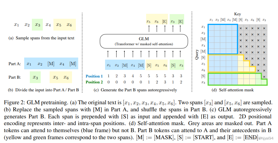
Part A tokens can attend to each other, but cannot attend to any
tokens in B. Part B tokens can attend to Part A and antecedents in B,
but cannot attend to any subsequent tokens in B. To enable
autoregressive generation, each span is padded with special tokens
[START] and [END], for input and output respectively. In this way, our
model automatically learns a bidirectional encoder (for Part A) and a
unidirectional decoder (for Part B) in a unified model. （GLM, 2022）

A部分的token可以相互关注，但是不能关注到B部分的token。B部分的tokens 可以关注 A 和 B 中的前项，但不能关注 B 中的任何后续 tokens。