Ax+By+C=0 直线一般式拟合 c++/python

资料来源于https://www.codeproject.com/Articles/576228/Line-Fitting-in-Images-Using-Orthogonal-Linear-Reg

先行Mark，并附python代码。另如下https://blog.csdn.net/linxue968/article/details/19913661中提供的方法存在问题，已测试

(r*v-s*t)*A^2 + (s^2-t^2-r*u+r*w)*A*B - (r*v-s*t)*B^2 = 0.
   A^2 + [(s^2-t^2-r*u+r*w)/(r*v-s*t)]*A*B - B^2 = 0.

这两个方程存在问题，多次求解均出现最后这两个方程化简后形式一样，不能求解，不知道转载相关文章的有没有测试过，笔者用直线示例和sympy库已经进行了测试，证实存在一定问题。

Line Fitting in Images Using Orthogonal Linear Regression

Introduction

A project I was working recently required me to take an image, identify (curved) lines within that image, and then represent those lines as lists of (straight) line segments. This article is a simplified version of that code, to describe the principle of line fitting in images.

Background

Fitting lines to points is a complex problem with a long mathematical history. For the purpose of this article, points means pixels. But points could also be data obtained in a scientific experiment. In both cases, sometimes we want to find a line (either curved or straight) that fits those points as accurately as possible. Fitting a curved line to a set of points is much harder than fitting a straight line. It is almost certainly iterative. And it is too complex for this article. So we are going to stick to fitting a straight line to a set of points. Also, if we need to fit a curve, we can do it with straight line segments – by applying this algorithm to small windows in the image, and storing the curved line as a list of line segments. To keep things simple, this article is going to assume that we just need to identify a single straight line. So now we have defined the problem, we need to find a suitable solution. In this case, we are going to use Orthogonal Linear Regression.

Linear Regression

Linear regression is more commonly associated with scientific experiments. Typically in an experiment you would get a set of output data for a set of input data. If you're lucky there would be a linear relationship between the input data and output data. For example we could apply a voltage to a resistor and measure the current through it (OK, so not a very exciting experiment!). Our data might look like this:

Voltage (V)	Current (I)
1.0	0.20
1.5	0.29
2.0	0.44
3.0	0.62
4.0	0.77

We can plot this, and using any spreadsheet, find a straight line through the points. This looks like:

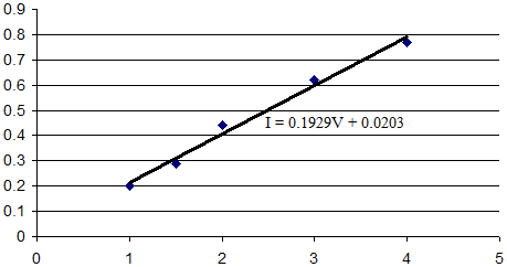
Spreadsheets generally use linear regression to calculate a straight trend line. The equation of this line is shown on the chart. 

We have to be careful how we interpret the result. In our case, since we know this is a resistor, the current at V = 0 should be 0, so we can be pretty certain that the intercept should be 0, not 0.0203. But there is also a more subtle issue. We might think we can flip the table (and the graph), so that we represent voltage against current:

Current (I)	Voltage (V)
0.20	1.0
0.29	1.5
0.44	2.0
0.62	3.0
0.77	4.0

If we plot this, we get:

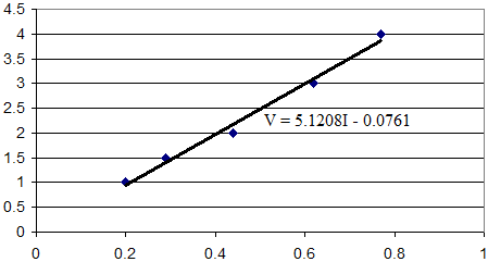
Now we can take the equation of this line and rearrange it to get I in terms of V. If we do this we get:

I = 0.1953V + 0.0149

Comparing this we our first graph, we can see that the equation is slightly different. Why? Well standard linear regression assumes that only only one variable (in this case the current) has errors. And that is how (simple) scientific experiments tend to work – we have one variable of our choice – and the other is measured. When we flip the table / chart, what we are actually saying is that the current is our choice, and the voltage is measured. This isn't what we did (actually we didn't do the first experiment either – I just made the numbers up! But the principle is valid).

So how does this relate to our problem of finding a line though a set of points? Well, in images we can't say that one axis is provided and the other is measured – both axes have errors in them. So when we look at the maths we find that the standard linear regression we used above won't work. We have to use another sort of linear regression called Errors In Variables (EIV) Linear Regression. This is a much more complex problem, and as it stands, not easily solvable. So there is one more assumption that we need to make – the errors in both variables are the same. This is important, and is true because X and Y are measured in the same units (pixels). Another important observation is that the errors that we are trying to minimise are perpendicular to the line that we are trying to fit. In standard linear regression the errors are perpendicular to the x axis. Hence our choice of Orthogonal Linear Regression.

The Formulas

The derivation of the formulas is quite involved, and covered in many papers, so I'm not going to go into detail here. Instead, I will just present the final solution.

The following equation will take the coordinates of a set of pixels as (x,y) pairs and find a line that fits those points (n = number of points). The equation of that line is going to be y = a + bx, where a is the intercept, and b is the slope. As part of the calculations we have to work out the following variables:

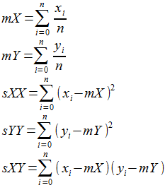
We then put those into the following equation:

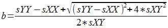
Now we have b, we can work out a by using:

The equations above are only valid if sXY is not equal to zero. If sXY is zero, then there are three possibilities:

1. We have a vertical line. This is the case if sXX < sYY.
2. We have a horizontal line. This is the case if sXX > sYY.
3. The line is indeterminate. This is the case if sXX == sYY.

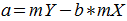
Vertical and horizontal lines are self explanatory. The simplest form of an indeterminate line is a single pixel. Clearly the line goes though the centre of the pixel, but it is impossible to say what the direction of the line is. Other combinations of pixels (e.g. 4 pixels in a tight square) will also have this property. Note that just because we can determine a line, it doesn't mean that we have a good line. Some examples of good lines are:

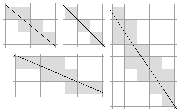
Some examples of bad lines are:

There are ways that we can determine if lines are a good fit or not. This is beyond the scope of this article. Instead we will assume that sensible arrangements of pixels are passed to the linear regression method. An approach that would help with this is to only use pixels that are adjacent to other pixels. This is also a sensible idea, since stray pixels can “drag” the line away from where it should be. This is because we are using a “least squares” method for minimising the errors. Although other approaches can be used, least squares ensures a very robust algorithm.

The Line Equation

There are various ways that we can represent lines. Up until the 1980s the slope / intercept form was very common. Even now, it is often taught to students. This may be because it is easy to visualise. It does however have a serious limitation – it doesn't work for vertical lines. Because of this, a more commonly used form is Ax + By = C. This works for all lines. One small issue is that there are infinitely many values of A, B and C for each line (e.g. 2x + 3y = 5 is the same line as 4x + 6y = 10). So we can't compare lines directly. There are various approaches we can take to normalise the line equation, which also ensure that the coefficients don't become very big or very small numbers. The normalisation that we will use is to ensure that C is positive, and that A2 + B2 = 1.0.

The Code

I have implemented the entire program as WinForms application. Since the important part of this article is the orthogonal linear regression calculation this is in a library of its own – Regression. The pixels are passed to the regression method via the interface IPixelGrid, which provides a simple way to access individual pixels. The CalculateLineEquation method takes a pixel grid as an input. The other input parameters are thae starting point (x and y) and width and height to use. The method returns the three line equation coefficients, a, b and c

public static void CalculateLineEquation(IPixelGrid grid, int x, int y, int width, int height,
                                         out float a, out float b, out float c)
{
    a = 0.0f;
    b = 0.0f;
    c = 0.0f;

    int n = 0, sX = 0, sY = 0;
    double mX, mY, sXX = 0.0, sXY = 0.0, sYY = 0.0;

    //Calculate sums of X and Y
    for (int iy = y; iy < y + height; iy++)
    {
        for (int ix = x; ix < x + width; ix++)
        {
            if (grid.GetPixel(ix, iy))
            {
                n++;
                sX += ix;
                sY += iy;
            }
        }
    }

    //Calculate X and Y means (sample means)
    mX = (double)sX / n;
    mY = (double)sY / n;

    //Calculate sum of X squared, sum of Y squared and sum of X * Y
    //(components of the scatter matrix)
    for (int iy = y; iy < y + height; iy++)
    {
        for (int ix = x; ix < x + width; ix++)
        {
            if (grid.GetPixel(ix, iy))
            {
                sXX += ((double)ix - mX) * ((double)ix - mX);
                sXY += ((double)ix - mX) * ((double)iy - mY);
                sYY += ((double)iy - mY) * ((double)iy - mY);
            }
        }
    }

    bool isVertical = sXY == 0 && sXX < sYY;
    bool isHorizontal = sXY == 0 && sXX > sYY;
    bool isIndeterminate = sXY == 0 && sXX == sYY;
    double slope = double.NaN;
    double intercept = double.NaN;

    if (isVertical)
    {
        a = 1.0f;
        b = 0.0f;
        c = (float)mX;
    }
    else if (isHorizontal)
    {
        a = 0.0f;
        b = 1.0f;
        c = (float)mY;
    }
    else if (isIndeterminate)
    {
        a = float.NaN;
        b = float.NaN;
        c = float.NaN;
    }
    else
    {
        slope = (sYY - sXX + Math.Sqrt((sYY - sXX) * (sYY - sXX) + 4.0 * sXY * sXY)) / (2.0 * sXY);
        intercept = mY - slope * mX;
        double normFactor = (intercept >= 0.0 ? 1.0 : -1.0) * Math.Sqrt(slope * slope + 1.0);
        a = (float)(-slope / normFactor);
        b = (float)(1.0 / normFactor);
        c = (float)(intercept / normFactor);
    }
}

The main form (MainForm) has a user control (PixelGridUserControl) to display the pixels, and allow the user to toggle pixels on or off. Once we have worked out the line (in terms of Ax+By=C), we can call the DrawLine method to display this. Note that because we are drawing pixels as large squares (and the centre of the pixel is the centre of the square), the edge of the displayed grid is actually half a pixel more than we would expect. So the displayed origin is actually (-0.5,-0.5) for example (when we later draw this line, we have to work out how big the squares are for each pixel – and will very depending on how much we have resized the form).

Note: If you want to make the displayed pixel grid bigger or smaller there is a constant in thePixelGridUserControl, NUM_PIXELS. By default this is set to 10, but can be between 2 and 500 (although I wouldn't recommend more than 50! - I haven't attempted to make it work well for big grids).

There is also a test library. By default this is not included in the build. If used, NUnit 2.6 needs to be installed.

Points Of Interest

This algorithm will almost certainly be a part of a bigger solution. Typically, an image will first have to be processed to extract lines or edges. The type of initial processing will be very dependant on the application.

Once you have the lines, you will typically have to use geometrical routines on these lines, such as working out where lines intersect, angles between lines, determining shapes etc. If I get enough interest in this article I may write follow up articles that show how some of these geometric calculations can be implemented.

References 

• Linear Regression (Wikipedia)
• Circular and Linear Regression: Fitting Circles and Lines by Least Squares (Nikolai Chernov)

Ax+By+C=0 直线一般式拟合Python实现代码

def generalLineFitParam(x,y):
    n=len(x)
    mX=sum(x)/n
    mY=sum(y)/n
    sXX=sum((np.array(x)-mX)**2)
    sYY=sum((np.array(y)-mY)**2)
    sXY=sum((np.array(x)-mX)*(np.array(y)-mY))
    
    if sXY ==0 and sXX<sYY:
        isVertical=True
    else:
        isVertical=False
    
    if sXY ==0 and sXX>sYY:
        isHorizontal=True
    else:
        isHorizontal=False
    
    if sXY ==0 and sXX==sYY:
        isIndeterminate=True
    else:
        isIndeterminate=False
    
    a=0.0;b=0.0;c=0.0;
    
    if isVertical:
        a=1.0
        b=0.0
        c=-mX
    elif isHorizontal:
        a=0.0
        b=1.0
        c=-mY
    elif isIndeterminate:
        a=np.NaN
        b=np.NaN
        c=np.NaN
    else:
        slope = (sYY - sXX + ((sYY - sXX) * (sYY - sXX) + 4.0 * sXY * sXY)**0.5) / (2.0 * sXY);
        intercept = mY - slope * mX;
        if intercept >=0:
            kFactors=1
        else:
            kFactors=-1
        normFactor = kFactors * (slope * slope + 1.0)**0.5;
        a = (float)(-slope / normFactor);
        b = (float)(1.0 / normFactor);
        c = (float)(intercept / normFactor);
    print("Line Param:a %f, b %f, c %f"%(a,b,c))
    
    return a, b, c

调用示例

x
Out[231]: [1, 1, 1]

y
Out[232]: [-1, -2, -3]

generalLineFitParam(x,y)
Line Param:a 1.000000, b 0.000000, c -1.000000
Out[233]: (1.0, 0.0, -1.0)

 

如下方评论（@guet_gjl）所说，上述方法得到的值存在不准确情况，所以如下为改进后的拟合程序（也是博主实际使用的方法），改进是判断拟合的目标直线是否是垂直于x轴，y轴，如果不是则采用正常sklearn 的liner_model进行拟合（记得import 相关包）。

def linerRegressionPredict(x, y):
    lr=linear_model.LinearRegression()
    lr.fit(x, y)
    #print('k:%f, b:%f'%( lr.coef_, lr.intercept_))
    return  lr

def calcLineSegmentLength(x,y):
    x1=x[0]
    y1=y[0]
    x2=x[len(x)-1]
    y2=y[len(y)-1]
    length=((x1-x2)**2+(y1-y2)**2)**0.5
    #print("Line segment length:",length)
    return length

def generalLineFitParam(x,y):
    n=len(x)
    mX=sum(x)/n
    mY=sum(y)/n
    sXX=sum((np.array(x)-mX)**2)
    sYY=sum((np.array(y)-mY)**2)
    sXY=sum((np.array(x)-mX)*(np.array(y)-mY))
    
    if sXY ==0 and sXX<sYY:
        isVertical=True
    else:
        isVertical=False
    
    if sXY ==0 and sXX>sYY:
        isHorizontal=True
    else:
        isHorizontal=False
    
    if sXY ==0 and sXX==sYY:
        isIndeterminate=True
    else:
        isIndeterminate=False
    
    a=0.0;b=0.0;c=0.0;
    
    if isVertical:
        a=1.0
        b=0.0
        c=-mX
    elif isHorizontal:
        a=0.0
        b=1.0
        c=-mY
    elif isIndeterminate:
        a=np.NaN
        b=np.NaN
        c=np.NaN
    else:
        #slope = (sYY - sXX + ((sYY - sXX) * (sYY - sXX) + 4.0 * sXY * sXY)**0.5) / (2.0 * sXY);
        #intercept = mY - slope * mX;
        X=np.array(x).reshape(len(x),1)#一维列表转为二维列表 
        Y=np.array(y).reshape(len(y),1)
        lr=linerRegressionPredict(X, Y)
        slope=lr.coef_[0][0]
        intercept=lr.intercept_[0]
        
        a = slope;
        b = -1;
        c = intercept;
    #print("Line Param:a %f, b %f, c %f"%(a,b,c))
    
    return a, b, c