


1. VAE的本质
1.1 深度理解VAE
-
VAE本质就是在我们常规的自编码器的基础上,对
encoder的结果(在VAE中对应着计算均值的网络)加上了 “ 高 斯 噪 声 ” \color{red}“高斯噪声” “高斯噪声”, 使 得 结 果 d e c o d e r 能 够 对 噪 声 有 鲁 棒 性 \color{red}使得结果decoder能够对噪声有鲁棒性 使得结果decoder能够对噪声有鲁棒性;而那个额外的KL loss(目的是让均值为0,方差为1),事实上就是相当于对encoder的一个正则项,希望encoder出来的东西均有零均值。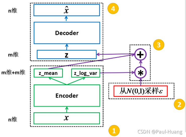
-
VAE 中的
encoder(对应着计算方差的网络)的作用:是用来 动 态 调 节 噪 声 的 强 度 \color{red}动态调节噪声的强度 动态调节噪声的强度的。- 当
decoder还没有训练好时( 重 构 误 差 \color{blue}重构误差 重构误差远大于KL loss),就会适当 降 低 噪 声 \color{blue}降低噪声 降低噪声(KL loss增加),使得拟合起来容易一些(重构误差开始下降); - 如果
decoder训练得还不错时( 重 构 误 差 \color{blue}重构误差 重构误差小于KL loss),这时 噪 声 就 会 增 加 \color{blue}噪声就会增加 噪声就会增加(KL loss减少),使得拟合更加困难了(重构误差又开始增加),这时候decoder就要想办法提高它的生成能力了。
具体理解参照:下图,以及以下公式
-
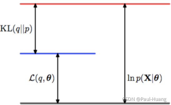
观测数据集 X = { x ( i ) } i = 1 N i . i . d X=\left\{ \mathtt{x}^{(i)} \right\}^N_{i=1} i.i.d X={x(i)}i=1Ni.i.d( X X X本身可能是连续分布或者离散分布),对某个 x x x的概率处理:
log p θ ( x ( i ) ) = log p θ ( x ( i ) , z ) − log p θ ( z ∣ x ( i ) ) = log p θ ( x ( i ) , z ) q ϕ ( z ∣ x ( i ) ) − log p θ ( z ∣ x ( i ) ) q ϕ ( z ∣ x ( i ) ) ( q ϕ ( z ∣ x ( i ) ) ≠ 0 ) . (1.1) \begin{aligned}\log\; p_{\theta}(\mathtt{x}^{(i)} )&=\log\; p_{\theta }(\mathtt{x}^{(i)},\mathtt{z})- \log\; p_{\theta }(\mathtt{z}|\mathtt{x}^{(i)})\\ &=\log\; \frac{p_{\theta }(\mathtt{x}^{(i)},\mathtt{z})}{q_{\phi}(\mathtt{z}|\mathtt{x}^{(i)})}-\log\; \frac{p_{\theta }(\mathtt{z}|\mathtt{x}^{(i)})}{q_{\phi}(\mathtt{z}|\mathtt{x}^{(i)})}\; \; (q_{\phi}(\mathtt{z}|\mathtt{x}^{(i)})\neq 0).\end{aligned}\tag{1.1} logpθ(x(i))=logpθ(x(i),z)−logpθ(z∣x(i))=logqϕ(z∣x(i))pθ(x(i),z)−logqϕ(z∣x(i))pθ(z∣x(i))(qϕ(z∣x(i))=0).(1.1)
(2.2.2)式两边对 q ϕ ( z ∣ x ( i ) ) q_{\phi}(\mathtt{z}|\mathtt{x}^{(i)}) qϕ(z∣x(i))求期望得:
log p θ ( x ( i ) ) = D K L ( q ϕ ( z ∣ x ( i ) ) ∣ ∣ p θ ( z ∣ x ( i ) ) ) + L ( θ , ϕ ; x ( i ) ) (1.2) \log p_\theta(\mathtt{x}^{(i)})=D_{KL}{(q_{\phi}(\mathtt{z}|\mathtt{x}^{(i)})||p_{\theta }(\mathtt{z}|\mathtt{x}^{(i)}))}+\mathcal{L}(\theta,\phi;\mathtt{x}^{(i)})\tag{1.2} logpθ(x(i))=DKL(qϕ(z∣x(i))∣∣pθ(z∣x(i)))+L(θ,ϕ;x(i))(1.2)
其中:
{ L ( θ , ϕ ; x ( i ) ) = ∫ z q ϕ ( z ∣ x ( i ) ) log p θ ( z , x ( i ) ) q ϕ ( z ∣ x ( i ) ) d z D K L ( q ϕ ( z ∣ x ( i ) ) ∣ ∣ p θ ( z ∣ x ( i ) ) ) = − ∫ z q ϕ ( z ∣ x ( i ) ) log p θ ( z ∣ x ( i ) ) q ϕ ( z ∣ x ( i ) ) d z \color{blue}\{ \begin{aligned} \mathcal{L}(\theta,\phi;\mathtt{x}^{(i)})&=\int_z q_{\phi}(\mathtt{z}|\mathtt{x}^{(i)}) \log\ \frac{p_{\theta }(\mathtt{z},\mathtt{x}^{(i)})}{q_{\phi}(\mathtt{z}|\mathtt{x}^{(i)})}dz\\ D_{KL}{(q_{\phi}(\mathtt{z}|\mathtt{x}^{(i)})||p_{\theta }(\mathtt{z}|\mathtt{x}^{(i)}))}&= - \int_z q_{\phi}(\mathtt{z}|\mathtt{x}^{(i)})\log\ \frac{p_{\theta }(\mathtt{z}|\mathtt{x}^{(i)})}{q_{\phi}(\mathtt{z}|\mathtt{x}^{(i)})}dz \end{aligned} {L(θ,ϕ;x(i))DKL(qϕ(z∣x(i))∣∣pθ(z∣x(i)))=∫zqϕ(z∣x(i))log qϕ(z∣x(i))pθ(z,x(i))dz=−∫zqϕ(z∣x(i))log qϕ(z∣x(i))pθ(z∣x(i))dz
-
L ( θ , ϕ ; x ( i ) ) \mathcal{L}(\theta,\phi;\mathtt{x}^{(i)}) L(θ,ϕ;x(i))又可以写成:
L ~ B ( θ , ϕ ; x ( i ) ) ≃ 1 2 ∑ j = 1 J ( 1 + log ( ( σ j ( i ) ) 2 ) − ( μ j ( i ) ) 2 − ( σ j ( i ) ) 2 ) ⏟ R e g u l a r i z a t i o n L o s s + 1 L ∑ l = 1 L ( log p θ ( x ( i ) ∣ z ( i , l ) ) ) ⏟ R e c o n s t r u c t i o n L o s s w h e r e z ( i , l ) = g ϕ ( x ( i ) , ϵ ( l ) ) = μ ( i ) + σ ( i ) ⊙ ϵ ( l ) a n d ϵ ( l ) ∼ N ( 0 , I ) (1.3) \color{red}\begin{aligned}&\widetilde{\mathcal{L}}^{B}\left(\boldsymbol{\theta}, \boldsymbol{\phi} ; \mathbf{x}^{(i)}\right)\simeq \underbrace{\frac{1}{2} \sum_{j=1}^{J}\left(1+\log \left(\left(\sigma_{j}^{(i)}\right)^{2}\right)-\left(\mu_{j}^{(i)}\right)^{2}-\left(\sigma_{j}^{(i)}\right)^{2}\right)}_{Regularization\;Loss}+\underbrace{\frac{1}{L} \sum_{l=1}^{L}\left(\log p_{\boldsymbol{\theta}}\left(\mathbf{x}^{(i)} \mid \mathbf{z}^{(i, l)}\right)\right)}_{Reconstruction\;Loss}\\ &where \quad\mathbf{z}^{(i,l)}=g_\phi(\mathbf{x}^{(i)},\epsilon^{(l)})=\boldsymbol{\mu}^{(i)} + \boldsymbol{\sigma^{(i)}}\odot \epsilon^{(l)} \quad and \quad \boldsymbol{\epsilon}^{(l)} \sim \mathcal{N}(\mathbf{0},\mathbf{I})\end{aligned}\tag{1.3} L B(θ,ϕ;x(i))≃RegularizationLoss 21j=1∑J(1+log((σj(i))2)−(μj(i))2−(σj(i))2)+ReconstructionLoss L1l=1∑L(logpθ(x(i)∣z(i,l)))wherez(i,l)=gϕ(x(i),ϵ(l))=μ(i)+σ(i)⊙ϵ(l)andϵ(l)∼N(0,I)(1.3)具体符号意义见:【论文阅读】生成模型——变分自编码器(Variational Auto-Encoder,VAE)公式(3.1.6)
- 当
1.2 VAE 与GAN
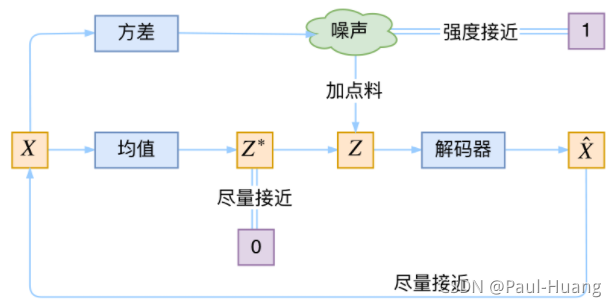
- VAE的对抗性
VAE中 重 构 的 过 程 是 希 望 没 噪 声 的 \color{red}重构的过程是希望没噪声的 重构的过程是希望没噪声的,而 K L l o s s 则 希 望 有 高 斯 噪 声 的 \color{red}KL loss则希望有高斯噪声的 KLloss则希望有高斯噪声的, 两 者 是 对 立 的 \color{red}两者是对立的 两者是对立的。所以,VAE跟GAN一样,内部其实是包含了一个对抗的过程,只不过它们两者是混合起来,共同进化的。 - VAE与GAN
- VAE是共同进化
- GAN的特点
- G A N 中 , 造 假 者 在 进 化 时 , 鉴 别 者 是 安 然 不 动 的 , 反 之 亦 然 。 \color{red}GAN中,造假者在进化时,鉴别者是安然不动的,反之亦然。 GAN中,造假者在进化时,鉴别者是安然不动的,反之亦然。
- GAN真正高明的地方是: 连 度 量 都 直 接 训 练 出 来 了 , 而 且 这 个 度 量 往 往 比 人 工 想 的 要 好 。 \color{red}连度量都直接训练出来了,而且这个度量往往比人工想的要好。 连度量都直接训练出来了,而且这个度量往往比人工想的要好。
- VAE的准确性
每个 p ( Z ∣ X ) p(Z|X) p(Z∣X)是不可能完全精确等于标准正态分布,否则 p ( Z ∣ X ) p(Z|X) p(Z∣X)就相当于跟 X X X无关了,重构效果将会极差。最终的结果就会是, p ( Z ∣ X ) p(Z|X) p(Z∣X)保留了一定的 X X X信息,重构效果也还可以,并且下式近似成立,所以同时保留着生成能力。
p ( Z ) = ∑ X p ( Z ∣ X ) p ( X ) = ∑ X N ( 0 , I ) p ( X ) = N ( 0 , I ) ∑ X p ( X ) = N ( 0 , I ) (1.4) p(Z)=\sum_{X} p(Z \mid X) p(X)=\sum_{X} \mathcal{N}(0, I) p(X)=\mathcal{N}(0, I) \sum_{X} p(X)=\mathcal{N}(0, I)\tag{1.4} p(Z)=X∑p(Z∣X)p(X)=X∑N(0,I)p(X)=N(0,I)X∑p(X)=N(0,I)(1.4)
2. CVAE
2.1 CVAE简介
-
VAE是无监督训练的,因此很自然想到:如果有标签数据,那么能不能把标签信息加进去辅助生成样本呢?这个问题的意图,往往是希望能够实现控制某个变量来实现生成某一类图像。当然,这是肯定可以的,我们把这种情况叫做Conditional VAE,或者叫CVAE。(相应地,在GAN中我们也有个CGAN。)
-
但是, C V A E 不 是 一 个 特 定 的 模 型 , 而 是 一 类 模 型 \color{red}CVAE不是一个特定的模型,而是一类模型 CVAE不是一个特定的模型,而是一类模型,总之就是 把 标 签 信 息 融 入 到 V A E 中 的 方 式 有 很 多 , 目 的 也 不 一 样 \color{red}把标签信息融入到VAE中的方式有很多,目的也不一样 把标签信息融入到VAE中的方式有很多,目的也不一样。这里基于前面的讨论,给出一种非常简单的VAE。
2.2 CVAE基本模型
- VAE与CVAE对比
- VAE基本模型:
- CVAE基本模型:
- VAE基本模型:
2.3 数学理解
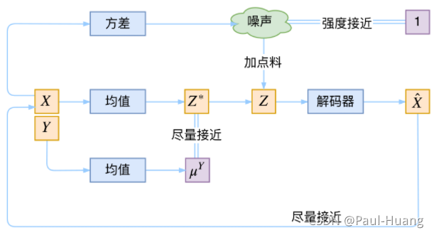
- VAE中希望
X
X
X经过编码后,
Z
Z
Z的分布都具有零均值和单位方差,这个“希望”是通过加入了
KL loss来实现的。如果现在多了类别信息 Y Y Y。 - CVAE希望同一个类的样本都有一个专属的均值 μ Y μ^Y μY(方差不变,还是单位方差),这个 μ Y μ^Y μY让模型自己训练出来。这样的话,有多少个类就有多少个正态分布,而在生成的时候,我们就可以通过控制均值来控制生成图像的类别。
- 事实上,这样可能也是在VAE的基础上加入最少的代码来实现CVAE的方案了,因为这个“新希望”也只需通过修改
KL loss实现:
L ~ B ( θ , ϕ ; x ( i ) ) ≃ 1 2 ∑ j = 1 J ( 1 + log ( ( σ j ( i ) ) 2 ) − ( μ j ( i ) − μ j Y ( i ) ) 2 − ( σ j ( i ) ) 2 ) ⏟ R e g u l a r i z a t i o n L o s s + 1 L ∑ l = 1 L ( log p θ ( x ( i ) ∣ z ( i , l ) ) ) ⏟ R e c o n s t r u c t i o n L o s s w h e r e z ( i , l ) = g ϕ ( x ( i ) , ϵ ( l ) ) = μ ( i ) + σ ( i ) ⊙ ϵ ( l ) a n d ϵ ( l ) ∼ N ( 0 , I ) (2.1) \color{red}\begin{aligned}&\widetilde{\mathcal{L}}^{B}\left(\boldsymbol{\theta}, \boldsymbol{\phi} ; \mathbf{x}^{(i)}\right)\simeq \underbrace{\frac{1}{2} \sum_{j=1}^{J}\left(1+\log \left(\left(\sigma_{j}^{(i)}\right)^{2}\right)-\left(\mu_{j}^{(i)}-\mu_{j}^{Y^{(i)}}\right)^{2}-\left(\sigma_{j}^{(i)}\right)^{2}\right)}_{Regularization\;Loss}+\underbrace{\frac{1}{L} \sum_{l=1}^{L}\left(\log p_{\boldsymbol{\theta}}\left(\mathbf{x}^{(i)} \mid \mathbf{z}^{(i, l)}\right)\right)}_{Reconstruction\;Loss}\\ &where \quad\mathbf{z}^{(i,l)}=g_\phi(\mathbf{x}^{(i)},\epsilon^{(l)})=\boldsymbol{\mu}^{(i)} + \boldsymbol{\sigma^{(i)}}\odot \epsilon^{(l)} \quad and \quad \boldsymbol{\epsilon}^{(l)} \sim \mathcal{N}(\mathbf{0},\mathbf{I})\end{aligned}\tag{2.1} L B(θ,ϕ;x(i))≃RegularizationLoss 21j=1∑J(1+log((σj(i))2)−(μj(i)−μjY(i))2−(σj(i))2)+ReconstructionLoss L1l=1∑L(logpθ(x(i)∣z(i,l)))wherez(i,l)=gϕ(x(i),ϵ(l))=μ(i)+σ(i)⊙ϵ(l)andϵ(l)∼N(0,I)(2.1)
更多内容,参考:CVAE


 702
702

 被折叠的 条评论
为什么被折叠?
被折叠的 条评论
为什么被折叠?
 到【灌水乐园】发言


