pcpnet：从原始点云学习局部形状属性

Abstract
In this paper, we propose PCPNET, a deep-learning based approach for estimating local 3D shape properties in point clouds.

In contrast to the majority of prior techniques that concentrate on global or mid-level attributes, e.g., for shape classification or semantic labeling, we suggest a patch-based learning method, in which a series of local patches at multiple scales around each point is encoded in a structured manner. Our approach is especially well-adapted for estimating local shape properties such as normals (both unoriented and oriented) and curvature from raw point clouds in the presence of strong noise and multi-scale features. Our main contributions include both a novel multi-scale variant of the recently proposed PointNet architecture with emphasis on local shape information, and a series of novel applications in which we demonstrate how learning from training data arising from well-structured triangle meshes, and applying the trained model to noisy point clouds can produce superior results compared to specialized state-of-the-art techniques. Finally, we demonstrate the utility of our approach in the context of shape reconstruction, by showing how it can be used to extract normal orientation information from point clouds.

在本文中，我们提出了一种基于深度学习的PCPNET方法，用于估计点云中的局部三维形状属性。（中心思想）

摘要
与大多数先前**专注于全局或中级属性的技术(**例如，用于形状分类或语义标记)相反，我们提出了一种基于补丁的学习方法，其中以结构化的方式编码每个点周围的多个尺度的一系列局部补丁。我们的方法特别适用于估计局部形状属性，如法线(无方向和有方向)和曲率，来自存在强噪声和多尺度特征的原始点云。我们的主要贡献包括最近提出的强调局部形状信息的PointNet架构的新颖多尺度变体，以及一系列新颖的应用，其中我们展示了如何从结构良好的三角形网格中产生的训练数据中学习，并将训练模型应用于嘈杂的点云，与专业的最新技术相比，可以产生更好的结果。最后，我们展示了我们的方法在形状重建的背景下的实用性，展示了如何使用它从点云中提取法线方向信息。
（知识点补充：点云的法线和曲率
在点云处理中，法线和曲率是两个重要的概念，用于描述点云中的表面特性和几何形状。

1. 法线（Normals）：
   **法线是指在给定点上表面的垂直方向。对于点云中的每个点，可以通过分析其周围的邻近点来估计该点的法线方向。**一种常用的方法是使用最近邻搜索或基于协方差矩阵的方法来计算每个点的法线。法线的表示通常是一个三维向量，它指示了点云表面在该点处的方向。法线在计算机图形学、计算机视觉以及三维重建等领域都有广泛的应用。

2. 曲率（Curvature）：
   **曲率用于描述点云表面在某个点处的弯曲程度。曲率是法线向量随着距离增加而变化的速率。在点云中，曲率可以提供关于表面形状的重要信息，例如表面的平坦区域和细节区域。**曲率的高值通常表示表面的弯曲或细节，而低值表示表面的平坦区域。计算曲率通常涉及对点云数据进行拟合或近似，以估计每个点处的曲率值。

法线和曲率在许多点云处理任务中都是很有用的特征。例如，当进行点云分割、特征提取、物体识别或表面重建时，这些特征可以帮助理解点云数据的结构和形状。同时，它们也为点云数据的可视化和分析提供了重要的信息。
）
Introduction
A fundamental problem in shape analysis is to robustly estimate local shape properties directly from raw point clouds. Although the problem has been extensively researched, a unified method that is robust under various data imperfections (e.g., varying noise level, sampling density, level of details, missing data) remains elusive.

In the context of continuous surfaces, local surface properties such as normals and curvature are classical differential geometric notions [dC76] and are known to uniquely characterize local geometry up to rigid transformations. In the context of discrete surfaces (e.g., polygonal meshes), the estimation methods fall broadly in two groups: evaluate normal/curvatures using discrete differential geometry operators, or use local primitive fitting and ‘read off’ normal/curvatures using attributes from the fitted primitives.

In the case of point clouds, a first challenge is the lack of connectivity information. Further, in real acquisition setups (e.g., using a depth camera), the data is often noisy, incomplete, and typically exhibit varying sampling density (based on scanning direction). Figure 1 shows a typical raw point cloud scan. The usual approach is to first locally define a neigborhood around each point using a rradius ball, and then fit a local primitive (e.g., plane or quadric surface) to the neighboring points. Although the method is simple and regularly used, in practice, the challenge is to appropriately pick the various parameters. For example, while it is desirable to pick a small value of r to avoid smoothing out sharp features, the same parameter can lead to unstable results in the presence of noise.

a large value of r can over-smooth local features, although the estimated values tend to be more stable under noise. The key challenge for such fitting-based methods is to manually set the various parameters depending on the (unknown) feature distribution in shapes and (unknown) noise margins in the raw scans.

介绍
**形状分析中的一个基本问题是直接从原始点云中鲁棒估计局部形状属性。**尽管这个问题已经得到了广泛的研究，但在各种数据缺陷(如不同的噪声水平、采样密度、细节水平、缺失数据)下，仍然难以找到一种统一的鲁棒方法。

在连续曲面的背景下，局部曲面性质，如法线和曲率是经典的微分几何概念[dC76]，并且已知是唯一表征局部几何直至刚性变换的特征。在离散曲面(例如多边形网格)的背景下，估计方法大致分为两组:使用离散微分几何算子评估法向/曲率，或使用局部原语拟合并使用拟合原语的属性“读取”法向/曲率。

在点云的情况下，第一个挑战是缺乏连接信息。此外，在实际采集设置中(例如，使用深度相机)，**数据通常是有噪声的，不完整的，并且通常表现出不同的采样密度(基于扫描方向)。**图1显示了一个典型的原始点云扫描。**通常的方法是首先使用半径球在每个点周围局部定义一个邻域，然后将局部原语(如平面或二次曲面)拟合到邻近点上。**虽然该方法简单且经常使用，但在实践中，挑战在于适当地选择各种参数。例如，**虽然我们希望挑选较小的r值可以避免平滑尖锐的特征，但是同样的参数在存在噪声的情况下会导致结果不稳定。
较大的r值可能会使局部特征过于平滑，尽管在噪声下估定值往往更稳定。**这种基于拟合的方法的关键挑战是根据(未知的)形状特征分布和原始扫描中的(未知的)噪声边缘手动设置各种参数。
（r值：采样的半径）

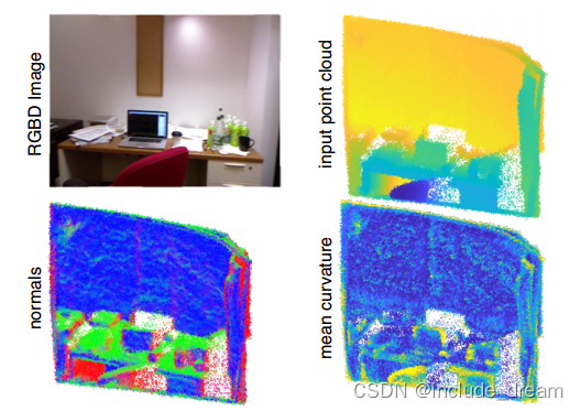
Our method can jointly estimate various surface properties like normals and curvature from noisy point sets. This scene is from the NYU dataset [NSF12] with added Gaussian noise and the bottom row shows properties estimated with PCPNET. Note that our method was not specifically trained on any RGBD dataset.

我们的方法可以从有噪声的点集中联合估计各种表面性质，如法线和曲率。这个场景来自NYU数据集[NSF12]，添加了高斯噪声，底部一行显示了用PCPNET估计的属性。请注意，我们的方法没有在任何RGBD数据集上进行专门训练。
（知识点补充：局部原语
在点云处理中，"局部原语"通常指代对点云中的局部区域进行基本操作的原始功能或基本操作。这些操作主要集中在点云的局部子集上，而不是整个点云。

以下是点云中常见的局部原语：

1. 点的选择：选择特定区域或一组点，以便在局部区域上执行后续操作。例如，基于距离阈值或几何属性来选择一组邻近的点。

2. 邻近搜索：查找每个点的近邻点集。邻近搜索是许多点云处理任务的基础，例如估计法线、曲率、表面重建等。

3. 采样：从点云中随机或均匀地选择点的子集。采样可以用于减少点云的密度，从而加快后续处理步骤。

4. 特征提取：从局部区域提取特征，用于描述该区域的几何和语义信息。例如，局部形状描述符用于表征点的局部几何结构。

5. 曲面拟合：将局部区域拟合为一个平面、曲线或曲面，以近似表示局部的几何形状。

6. 点云插值：使用局部邻近点来估计缺失的点或增加点的密度。

7. 点云滤波：对局部区域内的点进行滤波操作，例如移动平均滤波、高斯滤波等，用于去除噪声或平滑点云。

8. 特定任务的操作：根据具体的点云处理任务，还可以进行其他各种局部原语，例如点云配准、物体分割等。

总之，局部原语是在点云的局部区域内执行的基本操作，用于处理点云数据并提取局部信息，这些信息可以在许多点云处理任务中得到应用。）

In this work, we propose a data-driven approach for estimating local shape properties directly from raw pointclouds. In absence of local connectivity information, one could try to voxelize the occupied space, or establish local connectivity using k nearest neighbor graph. However, such discretizations introduce additional quantization errors leading to poor-quality local estimates. In an interesting recent work on normal estimation, Boulch et al [BM16] generate a set of local approximating planes, and then propose a data-driven denoising approach in the resultant Hough-space to estimate normals. In Section 5, we demonstrate that even such a specialized approach leads to errors on raw point clouds due to additional ambiguities introduced by the choice of the representation (RANSAClike Hough space voting).

Inspired by the recently introduced PointNet architecture [QSMG17] for shape classification and semantic segmentation, we propose a novel multi-scale architecture for robust estimation of local shape properties under a range of typical imperfections found in raw point clouds. Our key insight is that local shape properties can be robustly estimated by suitably accounting for shape features, noise margin, and sampling distributions. However, such a relation is complex, and difficult to manually account for. Hence, we propose a data-driven approach based on local point neighborhoods, wherein we train a neural network PCPNET to directly learn local properties (normals and curvatures) using groundtruth reference results under different input perturbations.

We evaluated PCPNET on various input point clouds and compared against a range of alternate specailized approaches. Our extensive tests indicate that PCPNET consistently produces superior normal/curvature estimates on raw point clouds in challenging scenarios. Specifically, the method is general (i.e., the same architecture simultaneously produces normal and curvature estimates), is robust to a range of noise margins and sampling variations, and preserves features around high-curvature regions. Finally, in a slightly surprising result, we demonstrate that a cascade of such local analysis (via the network depth) can learn to robustly extract oriented normals, which is a global property (similar patches may have opposite inside/outside directions in different shapes). Code for PCPNET is available at geometry.cs.ucl.ac.uk/projects/ 2018/pcpnet/.

在这项工作中，**我们提出了一种数据驱动的方法来直接从原始点云估计局部形状属性。**在缺乏本地连接信息的情况下，可以尝试将占用的空间体素化，或者使用k近邻图建立本地连接。然而，这种离散化引入了额外的量化误差，导致质量较差的局部估计。在最近一项关于法线估计的有趣研究中，Boulch等人[BM16]生成了一组局部逼近平面，然后在生成的hough空间中提出了一种数据驱动的去噪声方法来估计法线。在第5节中，我们证明了即使是这样一种专门的方法也会导致原始点云上的错误，这是由于选择表示(类似ransac的Hough空间投票)引入了额外的模糊性。

受最近引入的用于形状分类和语义分割的PointNet架构[QSMG17]的启发，我们提出了一种新的多尺度架构，**用于在原始点云中发现的一系列典型缺陷下对局部形状属性进行鲁棒估计。****我们的关键观点是，**局部形状属性可以通过适当地考虑形状特征、噪声裕度和采样分布来稳健地估计。然而，这样的关系是复杂的，并且很难手动解释。因此，我们提出了一种基于局部点邻域的数据驱动方法，其中我们训练了一个神经网络PCPNET，使用不同输入扰动下的真值参考结果直接学习局部属性(法线和曲率)。

我们在各种输入点云上评估了PCPNET，并与一系列替代的专门方法进行了比较。我们的广泛测试表明，PCPNET在具有挑战性的场景中始终对原始点云产生优越的法线/曲率估计。**具体来说，该方法是通用的(即，相同的架构同时产生法向和曲率估计)，对一系列噪声边缘和采样变化具有鲁棒性，并保留高曲率区域周围的特征。**最后，在一个稍微令人惊讶的结果中，我们证明了这种局部分析的级联(通过网络深度)可以学习鲁棒地提取定向法线，这是一个全局属性(类似的补丁可能在不同形状中具有相反的内/外方向)。PCPNET的代码可从geometry.cs.ucl.ac获得。英国/项目/ 2018 / pcpnet /。

Normal estimation. Estimating local differential information such as normals and curvature has a very long history in geometry processing, motivated in large part by its direct utility in shape reconstruction. Perhaps the simplest and best-known method for normal estimation is based on the classical Principal Component Analysis (PCA). This method, used as early as [HDD∗ 92], is based on analyzing the variance in a patch around a point and reporting the direction of minimal variance as the normal. It is extremely efficient, has been analyzed extensively, and its behavior in the presence of noise and curvature is well-understood [MNG04]. At the same time, it suffers from several key limitations: first it depends heavily on the choice of the neighborhood size, which can lead to oversmoothing for large regions or sensitivity to noise for small ones. Second, it is not well-adapted to deal with structured noise, and even the theoretical analysis does not apply in the case multiple, interacting, noisy shape regions, which can lead to non-local effects. Finally, it does not output the normal orientation since the eigenvectors of the covariance matrix are defined only up to sign.

Several methods have been proposed to address these limitations by both designing more robust estimation procedures, capable of handling more challenging data, and by proposing techniques for estimating normal orientation. The first category includes more robust distance-weighted approaches [PKKG03], methods such as osculating jets [CP03] based on fitting higher-order primitives robustly, the algebraic point set surface approach based on fitting algebraic spheres [GG07], approaches based on analyzing the distribution of Voronoi cells in the neighborhood of a point [AB99, ACSTD07, MOG11], and those based on edge-aware resampling [HWG∗ 13] among many others. Many of these techniques come with strong theoretical approximation and robustness guarantees (see e.g., Theorem 5.1 in [MOG11]). However, in practice they require a careful setting of parameters, and often depend on special treatment in the presence of strong or structured noise.

Unfortunately, there is no universal parameter set that would work for all settings and shape types.

Normal orientation. These challenges are arguably even more pronounced when trying to estimate oriented normals, since they depends on both local (for direction) and global (for orientation) shape properties. Early methods have relied on simple greedy orientation propagation, as done, for example in the seminal work on shape reconstruction [HDD∗ 92]. However, these approaches can easily fail in the presence of noisy normal estimates or high complexity shapes. As a result, they have has been extended significantly in recent years both through more robust estimates [HLZ∗ 09], which have also been adapted to handle large missing regions through point skeleton estimation [WHG∗ 15], and global techniques based on signed distance computations [MDGD∗ 10], among others. Nevertheless, reliably estimating oriented normals remains challenging especially across different noise levels and shape structures.

Curvature estimation. Similarly to surface normals, a large number of approaches has also been proposed for estimating principal curvatures. Several such techniques rely on estimating the normals first and then robustly fitting oriented curvatures [HM02, LP05], which in turn lead to estimates of principal curvature values. In a similar spirit, curvatures can be computed by considering normal variation in a local neighborhood [BC94, KNSS09]. While accurate in the presence of clean data, these techniques rely on surface normals, and any error is only be exacerbated by the further processing. One possible way to estimate the normal and the second fundamental form jointly is by directly fitting higher order polynomial as is done for example in the local jet fitting approach [CP03].

**法线估计。**估计局部微分信息(如法线和曲率)在几何处理中有很长的历史，很大程度上是由于它在形状重建中的直接应用。
也许最简单和最著名的正态估计方法是基于经典的主成分分析(PCA)。这种方法早在[HDD * 92]就开始使用了，它是基于分析一个点周围的斑块中的方差，并将最小方差的方向报告为正态。
（
PCA代表主成分分析（Principal Component Analysis），是一种常用的统计和机器学习技术，用于降维和数据压缩。它被广泛用于数据分析、特征提取和数据可视化等领域。

主成分分析的主要目标是将原始数据从高维空间转换为低维空间，同时尽可能保留数据的主要结构和信息。它通过找到数据中的主要方向（主成分），将数据投影到这些方向上，从而实现数据的降维。每个主成分都是原始数据中的线性组合，且彼此之间是正交的，从而确保了数据在低维空间中的最大可分性和信息保持。

主成分分析的基本步骤如下：

1. 去中心化：将原始数据的每个特征维度都减去其均值，使数据中心位于原点。

2. 计算协方差矩阵：计算去中心化后的数据的协方差矩阵。协方差矩阵反映了数据之间的相关性和变化情况。

3. 计算特征向量和特征值：对协方差矩阵进行特征分解，得到特征向量和特征值。特征向量表示主成分的方向，特征值表示数据在对应特征向量方向上的方差大小。

4. 选择主成分：根据特征值的大小，选择最重要的特征向量作为主成分。通常，特征值排序后，选择前面几个特征值对应的特征向量作为主成分。

5. 数据投影：将原始数据投影到选定的主成分上，得到降维后的数据。

主成分分析可以用于数据降维、特征提取、数据压缩和可视化。通过降低数据维度，可以减少计算和存储开销，并且在一些情况下，降维后的数据可以更好地用于后续的数据分析和模型建立。）

**它的效率极高，已被广泛分析，其在噪声和曲率存在下的行为也很好理解[MNG04]。**与此同时，它有几个关键的局限性:**首先，它严重依赖于邻域大小的选择，这可能导致大区域过平滑或小区域对噪声敏感。****其次，它不能很好地适应处理结构化噪声，甚至理论分析也不能适用于多个相互作用的噪声形状区域，这可能导致非局部效应。**最后，它不输出法向，因为协方差矩阵的特征向量只定义到符号。

已经提出了几种方法来解决这些限制，通过设计更健壮的估计程序，能够处理更具挑战性的数据，并通过提出估计法线方向的技术。第一类包括更鲁棒的距离加权方法[PKKG03]，基于鲁棒拟合高阶基元的密切喷射[CP03]，基于拟合代数球体的代数点集曲面方法[GG07]，基于分析点附近Voronoi细胞分布的方法[AB99, ACSTD07, MOG11]，以及基于边缘感知重采样的方法[HWG∗13]等等。这些技术中的许多都具有很强的理论近似性和鲁棒性保证(参见[MOG11]中的定理5.1)。然而，在实践中，它们需要仔细设置参数，并且通常依赖于在存在强噪声或结构化噪声时的特殊处理。

不幸的是，没有一个通用的参数集可以适用于所有的设置和形状类型。

法线方向。当尝试估计定向法线时，这些挑战可以说更加明显，因为它们依赖于局部(方向)和全局(方向)形状属性。
早期的方法依赖于简单的贪婪方向传播，例如在形状重建方面的开创性工作[HDD∗92]。然而，这些方法在存在噪声正态估计或高复杂性形状时很容易失败。因此，近年来通过更稳健的估计[HLZ∗09]，以及基于符号距离计算[MDGD∗10]的全局技术，它们已经得到了显著的扩展，这些估计也被适应于通过点骨架估计[WHG∗15]来处理大型缺失区域。然而，可靠地估计定向法线仍然具有挑战性，特别是在不同的噪声水平和形状结构中。

**曲率估算。**与曲面法线类似，也提出了大量估计主曲率的方法。**一些这样的技术依赖于首先估计法线，然后鲁棒拟合定向曲率[HM02, LP05]，这反过来导致主曲率值的估计。**同样，曲率也可以通过考虑局部邻域的正态变化来计算[BC94, KNSS09]。**虽然在干净的数据下是准确的，但这些技术依赖于表面法线，任何错误都只会在进一步处理时加剧。**一种可能同时估计法向和第二基本形式的方法是直接拟合高阶多项式，例如局部射流拟合方法[CP03]。
**（**知识点补充：STN
STN代表空间转换网络（Spatial Transformer Network），是一种在深度学习中用于增强模型空间不变性的网络结构。

STN最初由DeepMind的Jaderberg等人在2015年提出。它的主要目标是在神经网络中引入空间变换，使得模型可以自动学习对输入数据进行平移、缩放、旋转等几何变换，从而提高模型对于输入数据的鲁棒性和泛化能力。

STN的基本原理如下：

1. 空间变换：STN引入一个可学习的空间变换模块，用于对输入数据进行几何变换。该变换模块由神经网络组成，可以学习到输入数据的变换矩阵。

2. 网格生成：在空间变换模块中，通常会生成一个网格，用于描述输入数据的采样位置。这个网格的变换信息由网络学习得到。

3. 采样：通过应用学习到的变换矩阵，将网格中的点映射到输入数据上，得到经过空间变换的输出数据。

4. 整合到网络：STN的空间变换模块可以嵌入到其他神经网络模型中，例如卷积神经网络（CNN）或全连接神经网络。这样，整个网络可以端到端地学习输入数据的空间变换和任务相关特征。

STN的应用场景包括图像分类、目标检测、语义分割等。通过引入空间变换，STN可以使得模型对于输入数据的姿态变化和尺度变化具有一定的鲁棒性，从而提高模型在复杂场景下的性能表现。

总体而言，空间转换网络（STN）是一种在深度学习中引入空间变换的技术，用于增强模型对于输入数据的空间不变性，从而提高模型的鲁棒性和泛化能力。）

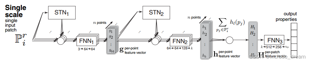
单尺度网络架构：

多尺度网络架构：

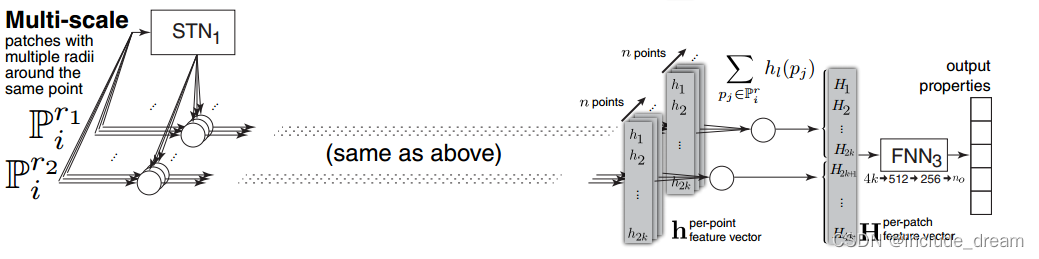
We propose two architectures for our network, a single- and a multi-scale architecture. In both architectures, the network learns a set of point functions h in the local space of a point set patch. Similar to a density estimator, point function values at each point in the patch are summed up. The resulting per-patch feature vector H can be used to regress patch properties. STNs are spatial transformer networks that apply either a quaternion rotation (STN1) or a full linear transformation (STN2). FNNs are fully connected networks. In the multi-scale architecture patches of different scale are treated as a single larger patch by the point functions. The final sum is performed separately for each patch.

我们为我们的网络提出了两种架构，单尺度架构和多尺度架构。在这两种体系结构中，网络在点集patch的局部空间中学习一组点函数h。与密度估计器类似，对patch中每个点的点函数值进行求和。得到的每个补丁特征向量H可用于回归补丁属性。stn是应用四元数旋转(STN1)或全线性变换(STN2)的空间变压器网络。fnn是全连通网络。在多尺度体系结构中，不同尺度的小块被点函数视为一个更大的小块。对每个补丁分别进行最终求和。

（知识点补充：FNN
FNN代表"Feedforward Neural Network"，中文翻译为前馈神经网络。它是一种最常见和基础的神经网络模型，也是深度学习中最早的模型之一。

前馈神经网络是一种全连接的神经网络，其中神经元按照层次结构排列。它包含一个输入层、若干个隐藏层和一个输出层。数据从输入层开始经过网络中的各个隐藏层，最终到达输出层，这样的传播过程是单向的，没有反馈回路，因此称之为前馈。

每个神经元与下一层中的所有神经元相连接，通过一系列权重和偏置来实现信息传递和处理。每个连接都有一个对应的权重，而每个神经元都会根据其输入和激活函数的输出计算出一个输出值。隐藏层和输出层中的每个神经元通常都具有非线性的激活函数，这样可以让前馈神经网络具备处理复杂非线性关系的能力。

前馈神经网络在深度学习中的应用非常广泛，包括图像分类、目标检测、自然语言处理等领域。由于其简单直观的结构和较强的能力，前馈神经网络为深度学习的发展奠定了基础，并为后续更复杂的神经网络模型提供了灵感和基础。
）
Deep Learning for Geometric Data

In the recent years, several methods have been proposed for analyzing and processing 3D shapes by building on the success of machine learning methods, and especially those based on deep learning (see, for example, recent overviews in [MRB∗ 16, BBL∗ 17]).

These methods are based on the notion that the solutions to many problems in geometric data analysis can benefit from large data repositories. Many learning-based approaches are aimed at estimating global properties for tasks such as shape classification and often are based either on 2D projections (views) of 3D shapes or on volumetric representations (see, e.g., [QSN∗ 16] for a comparison). However, several methods have also been proposed for shape segmentation [GZC15,MGA∗ 17] and even shape correspondence [MBBV15,WHC∗ 16,BMRB16], among many others.

Although most deep learning-based techniques for 3D shapes heavily exploit the mesh structure especially for defining convolution operations, few approaches have also been proposed to directly operate on point clouds. Perhaps the most closely related to ours are recent approaches of Boulch et al [BM16] and Qi et al [QSMG17].

The former propose an architecture for estimating unoriented normals on point clouds by creating a Hough transform-based representation of local shape patches and using a convolutional neural network for learning normal directions from a large ground-truth corpus. While not projection based, this method still relies on a 2D-based representation for learning and moreover loses orientation information, which can be crucial in practice. More recently, the PointNet architecture [QSMG17] has been designed to operate on 3D point clouds directly. This approach is very versatile as it allows to estimate properties of 3D shapes without relying on 2D projections or volumetric approximations. The original architecture is purely global, taking the entire point cloud into account, primarily targeting shape classification and semantic labeling, and has since then been extended to a hierarchical approach in a very recent PointNet++ [QYSG17], which is designed to better capture local structures in point clouds.

Our approach is based on the original PointNet architecture, but rather than using it for estimating global shape properties for shape classification or semantic labeling, as has also been the focus of PointNet++ [QYSG17], we adapt it explicitly for estimating local differential properties including oriented normals and curvature.

几何数据的深度学习：

近年来，基于机器学习方法的成功，特别是基于深度学习的方法，已经提出了几种分析和处理3D形状的方法(例如，参见[MRB∗16,BBL∗17]中的最近概述)。

这些方法基于这样一个概念，即几何数据分析中许多问题的解决方案可以从大型数据存储库中受益。许多基于学习的方法旨在估计诸如形状分类等任务的全局属性，并且通常基于3D形状的2D投影(视图)或体积表示(例如，参见[QSN∗16]进行比较)。然而，也有几种方法被提出用于形状分割[GZC15,MGA∗17]和甚至形状对应[MBBV15,WHC∗16,BMRB16]等。

尽管大多数基于深度学习的3D形状技术都大量利用网格结构，特别是在定义卷积操作时，但很少有方法可以直接对点云进行操作。也许与我们最密切相关的是Boulch等人[BM16]和Qi等人[QSMG17]最近的方法。

前者提出了一种估计点云上无方向法线的架构，通过创建基于Hough变换的局部形状斑块表示，并使用卷积神经网络从大型地基真语料库中学习法线方向。虽然不是基于投影的，但这种方法仍然依赖于基于2d的表示来学习，而且会丢失方向信息，这在实践中是至关重要的。最近，PointNet架构[QSMG17]被设计为直接在3D点云上操作。这种方法非常通用，因为它允许在不依赖于2D投影或体积近似的情况下估计3D形状的属性。最初的架构是完全全局的，考虑到整个点云，主要针对形状分类和语义标记，并在最近的PointNet++ [QYSG17]中扩展为分层方法，旨在更好地捕获点云中的局部结构。

我们的方法是基于原始的PointNet架构，但不是使用它来估计形状分类或语义标记的全局形状属性，这也是PointNet++ [QYSG17]的重点，我们明确地将其用于估计局部微分属性，包括定向法线和曲率。

Overview

Estimating local surface properties, such as normals or curvature, from noisy point clouds is a difficult problem that is traditionally solved by extracting these properties from smooth surfaces fitted to local patches of the point cloud. However these methods are sensitive to parameter settings such as the neighborhood size, or the degree of the fitted surface, that need to be carefully set in practice.

Instead, we propose an alternative approach that is robust to a wide range of conditions with the same parameter settings, based on a deep neural network trained on a relatively small set of shapes.

综述；概观

从噪声点云中估计局部表面属性(如法线或曲率)是一个难题，传统上通过从适合点云局部斑块的光滑表面提取这些属性来解决。然而，这些方法对参数设置很敏感，如邻域大小或拟合表面的程度，需要在实践中仔细设置。

相反，我们提出了一种替代方法，该方法基于在相对较小的形状集上训练的深度神经网络，具有相同参数设置的广泛条件的鲁棒性。

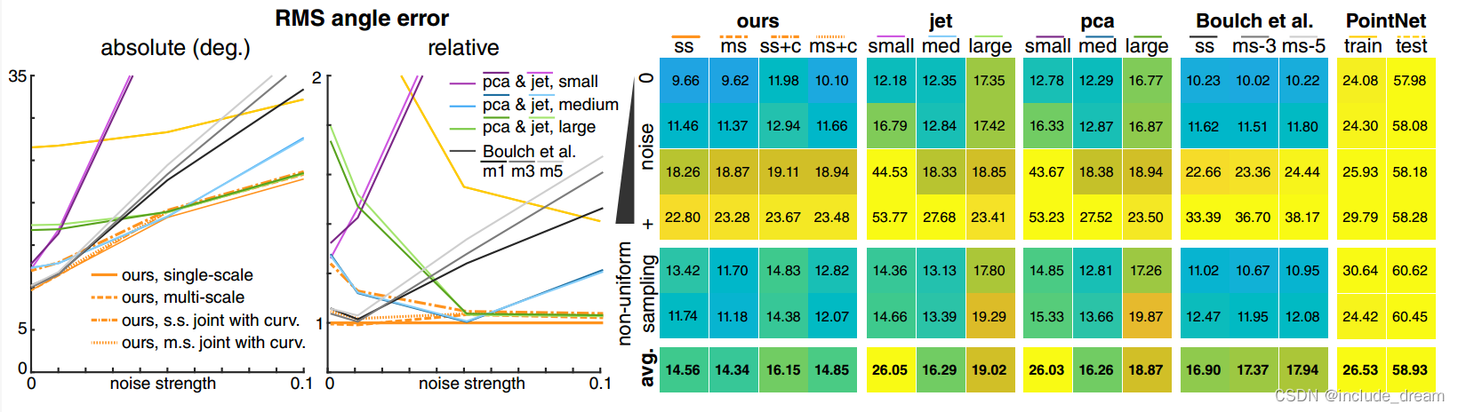
Comparison of the RMS normal angle error of our method (ss: single scale, ms: mult-scale, +c: joint normals and curvature) to geometric methods (jet fitting and PCA) with three patch sizes and two deep learning methods (Boulch et al [BM16] and PointNet [QSMG17]). Note that geometric methods require correct parameter settings, such as the patch size, to achieve good results. Our method gives good results without the need to adjust parameters.

我们的方法(ss:单尺度，ms:多尺度，+c:联合法线和曲率)与几何方法(射流拟合和PCA)在三种斑块大小和两种深度学习方法(Boulch et al [BM16]和PointNet [QSMG17])下的RMS法线角度误差的比较。请注意，几何方法需要正确的参数设置，例如补丁大小，以获得良好的结果。我们的方法在不需要调整参数的情况下得到了很好的结果。

Given a point cloud P = fp1;:::; pNg, our PCPNET network (see Figure 2 for an overview) is applied to local patches of this point cloud P r i 2 P, centered at points pi with a fixed radius r proportional to the point cloud’s bounding box extent. We then estimate local shape properties at the central points of these patches.

The architecture of our network is inspired by the recent PointNet [QSMG17], adapted to local r-neighborhood patches instead of the entire point cloud. The network learns a set of k non-linear functions in the local patch neighborhoods, which can intuitively be understood as a set of density estimators for different regions of the patch. These give a k-dimensional feature vector per patch that can then be used to regress various local features.

给定一个点云P = fp1;:::;pNg，我们的PCPNET网络(概观见图2)被应用于这个点云的局部补丁，以点pi为中心，固定半径r与点云的边界框范围成比例。然后我们估计这些斑块中心点的局部形状属性。

我们的网络架构受到最近的PointNet [QSMG17]的启发，适应于局部r邻域补丁而不是整个点云。网络在局部patch邻域中学习k个非线性函数，可以直观地理解为patch不同区域的密度估计量。这些给出了每个补丁的k维特征向量，然后可以用来回归各种局部特征。

Algorithm
Our goal in this work is to reconstruct local surface properties from a point cloud that approximately samples an unknown surface. In real-world settings, these point clouds typically originate from scans or stereo reconstructions and suffer from a wide range of deteriorating conditions, such as noise and varying sampling densities. Traditional geometric approaches for recovering surface properties usually perform reasonably well with the correct parameter settings, but finding these settings is a data-dependent and often difficult task. The success of deep-learning methods, on the other hand, is in part due to the fact that they can be made robust to a wide range of conditions with a single hyper-parameter setting, seemingly a natural fit to this problem. The current lack of deep learning solutions may be due to the difficulty of applying deep networks to unstructured input like point clouds. Simply inputting points as a list would make the subsequent computations dependent on the input ordering.

A possible solution to this problem was recently proposed under the name of PointNet by Qi et al [QSMG17], who propose combining input points with a symmetric operation to achieve orderindependence. However, PointNet is applied globally to the entire point cloud, and while the authors do demonstrate estimation of local surface properties as well, these results suffer from the global nature of the method. PointNet computes two types of features in a point cloud: a single global feature vector for the entire point cloud and a set of local features vectors for each point. The local feature vectors are based on the position of a single point only, and do not include any neighborhood information. This reliance on only either fully local or fully global feature vectors makes it hard to estimate properties that depend on local neighborhood information.

Instead, we propose computing local feature vectors that describe the local neighborhood around a point. These features are better suited to estimate local surface properties. In this section, we provide an alternative analysis of the PointNet architecture and show a variation of the method that can be applied to local patches instead of globally on the entire point cloud to get a strong performance increase for local surface property estimation, outperforming the current state-of-the art.

算法
在这项工作中，我们的目标是从一个近似采样未知表面的点云重建局部表面属性。在现实环境中，这些点云通常来自扫描或立体重建，并且受到各种恶化条件的影响，例如噪声和不同的采样密度。在正确的参数设置下，恢复表面性质的传统几何方法通常表现得相当好，但找到这些设置是一个依赖于数据的任务，而且往往是一项艰巨的任务。另一方面，深度学习方法的成功部分是因为它们可以通过单一的超参数设置对广泛的条件具有鲁棒性，这似乎是解决这个问题的自然选择。目前缺乏深度学习解决方案可能是由于将深度网络应用于点云等非结构化输入的困难。简单地以列表形式输入点会使后续计算依赖于输入顺序。

最近Qi等人[QSMG17]以PointNet的名义提出了一种可能的解决方案，他们提出将输入点与对称操作结合起来以实现顺序独立性。然而，PointNet是全局应用于整个点云的，虽然作者也演示了局部表面性质的估计，但这些结果受到该方法全局性质的影响。PointNet在点云中计算两种类型的特征:整个点云的单个全局特征向量和每个点的一组局部特征向量。局部特征向量仅基于单个点的位置，不包含任何邻域信息。这种仅依赖于完全局部或完全全局特征向量的情况使得难以估计依赖于局部邻域信息的属性。

相反，我们建议计算描述点周围局部邻域的局部特征向量。这些特征更适合于估计局部表面性质。在本节中，我们提供了对PointNet架构的另一种分析，并展示了该方法的一种变体，该方法可以应用于局部补丁，而不是全局地应用于整个点云，从而在局部表面属性估计方面获得了强大的性能提升，优于当前的最先进技术。
（PCPnet还是基于pointnet网络架构的）

Pre-processing

Given a point cloud P = fp1;:::; pNg, a local patch P r i is centered at point pi and contains all points within distance r from the center.

Our target for this patch are local surface properties such as normal ni and principal curvature values k 1 i and k 2 i at the center point pi .

To remove unnecessary degrees of freedom from the input space, we translate the patch to the origin and normalize its radius multiplying with 1/r. Since the curvature values depend on scale, we transform output curvatures to the original scale of the point cloud by multiplying with r. Our network takes a fixed number of points as input. Patches that have too few points are padded with zeros (the patch center), and we pick a random subset for patches with too many points.

预处理

给定一个点云P = fp1;:::;pNg，一个局部patch pi以点pi为中心，包含距离该中心距离为r的所有点。

我们的目标是局部表面属性，如法向ni和主曲率值k1 i和k2 i在中心点pi。

为了从输入空间中去除不必要的自由度，我们将patch平移到原点，并将其半径乘以1/r归一化。由于曲率值依赖于尺度，我们通过乘以r将输出曲率转换为点云的原始尺度。我们的网络将固定数量的点作为输入。点过少的补丁被0填充(补丁中心)，我们为有太多点的补丁选择一个随机子集。

Architecture

Our single-scale network follows the PointNet architecture, with two changes: we constrain the first spatial transformer to the domain of rotations and we exchange the max symmetric operation with a sum. An overview of the architecture is shown in Figure 2.

We will now provide intuition for this choice of architecture.

架构

我们的单尺度网络遵循PointNet架构，有两个变化:我们将第一个空间转换器约束到旋转域，并将最大对称操作与求和交换。该体系结构的概述如图2所示。

现在我们将为这种体系结构的选择提供直观的说明。

Quaternion spatial transformer.
The first step of the architecture transforms the input points to a canonical pose. This transformation is optimized for during training, using a spatial transformer network [JSZK15]. We constrain this transformation to rotations by outputting a quaternion instead of a 3 × 3 matrix. This is done for two reasons: First, unlike in semantic classification, our outputs are geometric properties that are sensitive to transformations of the patch. This caused unstable convergence behavior in early experiments where scaling would take on extreme values. Rotation-only constraints stabilized convergence. Second, we have to apply the inverse of this transformation to the final surface properties and computing the inverse of a rotation is trivial.

四元数空间转换器。
该体系结构的第一步是将输入点转换为规范姿态。在训练期间，使用空间变压器网络对这种转换进行优化[JSZK15]。我们将这个变换约束为旋转通过输出一个四元数而不是一个3 × 3矩阵。这样做有两个原因:首先，与语义分类不同，我们的输出是对patch转换敏感的几何属性。这在早期的实验中会导致不稳定的收敛行为，因为缩放会取极值。仅旋转约束稳定收敛。其次，我们必须将这个变换的逆应用到最终的表面性质中，计算旋转的逆是微不足道的。

Point functions and symmetric operation.

One important property of the network is that it should be invariant to the input point ordering. Qi et al [QSMG17] show that this can be achieved by applying a set of functions fh1;:::;hkg with shared parameters to each point separately and then combine the resulting values for each point using a symmetric operation:

点函数和对称运算。

该网络的一个重要性质是它对输入点的顺序是不变的。Qi等[QSMG17]表明，这可以通过对每个点分别应用一组具有共享参数的函数fh1;:::;hkg，然后使用对称操作将每个点的结果值组合起来来实现:

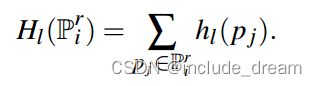
Hl(P r i ) is then a feature of the patch and hl are called point functions; they are scalar-valued functions, defined in the in the local coordinate frame of the patch. The functions Hl can intuitively be understood as density estimators for a region given by hl . Their response is stronger the more points are in the non-zero region of hl .

Compared to using the maximum as symmetric operation, as proposed by Qi et al, our sum did not have a significant performance difference; however we decided to use the sum to give our point functions a simple conceptual interpretation as density estimators.

The point functions hl are computed as:

Hl(pi)是patch的一个特征，Hl称为点函数;它们是标量值函数，定义在patch的局部坐标系中。函数Hl可以直观地理解为Hl给出的区域的密度估计量。它们的响应越强，点在hl的非零区域越多。

与Qi等人提出的使用最大值作为对称操作相比，我们的求和没有显著的性能差异;然而，我们决定使用求和来给我们的点函数一个简单的概念解释作为密度估计。

点函数hl计算为:

The second spatial transformer
operates on the feature vector gj = g1(pj);:::;g64(pj) , giving a 64×64 transformation matrix. Some insight can be gained by interpreting the transformation as a fully connected layer with weights that are computed from the feature vectors g of all points in the patch. This introduces global information into the point functions, increasing the performance of the network.

第二个空间转换器
作用于特征向量gj = g1(pj);:::;g64(pj) ，给出一个64×64变换矩阵。通过将转换解释为具有从patch中所有点的特征向量g计算的权重的完全连接层，可以获得一些见解。这将全局信息引入到点函数中，提高了网络的性能。

Output regression. In a trained model, the patch feature vector Hj = (H1(P r i );:::;Hk(P r i )) provides a rich description of the patch.

Various surface properties can be regressed from this feature vector. We use a three-layer fully connected network to perform this regression.

**输出回归。**在训练好的模型中，patch特征向量Hj = (H1(p1 i);:::;Hk(p1 i))提供了对patch的丰富描述。
各种表面属性可以从这个特征向量回归。我们使用三层全连接网络来执行此回归。（回归训练）

（知识点补充：向量回归
向量回归是一种机器学习任务，旨在通过输入特征来预测一个向量型的目标值。在传统的回归问题中，目标值通常是一个标量，即一个单一的数值，如房价预测、销售量预测等。而在向量回归中，目标值是一个向量，即包含多个数值的数据结构。

在向量回归中，我们有一组输入特征（通常表示为向量），通过训练模型，预测输出目标值也是一个向量。向量回归的目标是找到一个合适的函数关系，将输入特征映射到目标值的向量。

向量回归在各种应用场景中都有广泛的应用，特别是当需要同时预测多个相关目标值时。例如：

1. 多维时序预测：在时间序列预测任务中，可能需要同时预测多个相关的时间序列，如多个商品的销售量预测。

2. 多标签分类：在多标签分类任务中，每个样本可能对应多个标签，例如图像中的多个物体识别。

3. 多目标优化：在优化问题中，可能需要同时优化多个目标函数，例如在机器学习模型中考虑多个性能指标。

解决向量回归问题的方法类似于传统的回归问题，但需要注意输出层的设置和损失函数的选择，以适应目标值是向量的情况。

总的来说，向量回归是一种机器学习任务，用于通过输入特征预测一个向量型的目标值。它在许多领域中都有重要的应用，涉及到多目标预测和优化问题。）

Multi-scale

We will show in the results, that the architecture presented above is very robust to changes in noise strength and sample density. For additional robustness, we experimented with a multi-scale version of the architecture. Instead of using a single patch as input, we input three patches P r1 i , P r2 I and P r1 I with different radii. Due to the scale normalization of our patches, these are scaled to the same size, but contain differently sized regions of the point cloud. This allows all point functions to focus on the same region. We also triple the number of point functions, but apply each function to all three patches.

The sum however, is computed over each patch separately. This results in nine-fold increase in patch features H, which are then used to regress the output properties. Figure 2 illustrates a simple version of this architecture with two patches.

多尺度架构

我们将在结果中显示，上述架构对噪声强度和样本密度的变化非常稳健。为了获得额外的健壮性，我们尝试了该架构的多尺度版本。我们不使用单个patch作为输入，而是输入三个不同半径的patch pr1 i, pr2 i和pr1 i。由于我们的补丁的尺度归一化，这些被缩放到相同的大小，但包含不同大小的点云区域。这允许所有点函数聚焦于同一区域。我们还将点函数的数量增加了三倍，但将每个函数应用于所有三个补丁。
然而，总和是在每个补丁上分别计算的。这导致补丁特征H增加了9倍，然后用于回归输出属性。图2展示了该体系结构的一个简单版本，其中包含两个补丁。

Evaluation and Discussion

In this section, we evaluate our method in various settings and compare it to current state of the art methods. In particular, we compare our curvature estimation to the osculating jets method [CP03] and a baseline PCA method, and the normal estimation additionally to PointNet [QSMG17] and the normal estimation method of Boulch et al [BM16]. We test the performance of these methods on shapes with various noise levels and sampling rates, as described below. For the method of Boulch et al, we use the code and trained networks provided by the authors. PointNet has code, but no pre-trained network for normal estimation available, so we re-train on our dataset. For the other methods we use the implementation within CGAL [CGA].

评价与讨论

在本节中，我们将在各种设置中评估我们的方法，并将其与当前最先进的方法进行比较。特别地，我们将曲率估计与密切 jets 方法[CP03]和基线PCA方法进行了比较，并将正态估计与PointNet [QSMG17]和Boulch等[BM16]的正态估计方法进行了比较。我们测试了这些方法在不同噪声水平和采样率的形状上的性能，如下所述。对于Boulch等人的方法，我们使用了作者提供的代码和训练过的网络。PointNet有代码，但没有用于正常估计的预训练网络，所以我们在我们的数据集上重新训练。对于其他方法，我们使用CGAL [CGA]中的实现。

output 3D normals, curvatures, or both at the same time. We evaluate the performance of the network when trained separately for normals and curvatures or jointly using a single network for both outputs. We also compare the performance of a network trained with both curvature values against networks trained for individual curvature values.

输出3D法线，曲率，或两者在同一时间。我们分别对法线和曲率进行训练或对两个输出联合使用单个网络时，评估网络的性能。我们还比较了用两个曲率值训练的网络与用单个曲率值训练的网络的性能。

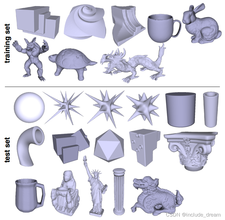
Our shape dataset. We train and test on a mix of simple shapes like the sphere or the boxes, and more detailed shapes like statues or figures. The test set additionally contains three analytic shapes not shown here (sphere, cylinder and a thin sheet shown in Figure 8).

我们的形状数据集。我们训练和测试的混合简单的形状，如球体或盒子，更详细的形状，如雕像或人物。测试集还包含三个解析形状(如图8所示的球体、圆柱体和薄片)。

Dataset

One of the advantages of training the network on point cloud patches rather than point clouds of complete shapes is that we can sample a large number of patches from each shape. Two patches with near-by center points may still be significantly different from each other in terms of the type of structure they contain, such as edges, corners, etc. Thus, we can use a relatively small dataset of labeled shapes to train our network effectively. Figure 5 shows the shapes in our dataset.

Our training dataset contains 8 shapes, half of which are man made objects or geometric constructs with flat faces and sharp corners, and the other half are scans of figurines (bunny, armadillo, dragon and turtle). All shapes are given as triangular meshes. We sample the faces of each mesh uniformly with 100000 points to generate a point cloud. Each of these 100000 points can be used as a patch center. We label each point with the normal of the face it was sampled from. We also estimate the k 1 and k 2 curvature values at the vertices and interpolate them for each sampled points.

The curvature estimation is performed using the method suggested by Rusinkiewicz in [Rus04] (the code was provided by authors of [SF15]).

数据集

**在点云小块而不是完整形状的点云上训练网络的一个优点是，我们可以从每个形状中抽取大量的小块。**中心点附近的两个斑块在其包含的结构类型(如边缘、角等)方面仍然可能存在显著差异。因此，我们可以使用一个相对较小的标记形状数据集来有效地训练我们的网络。图5显示了我们数据集中的形状。

我们的训练数据集包含8个形状，其中一半是人造物体或平面和尖角的几何结构，另一半是小雕像(兔子，犰狳，龙和乌龟)的扫描。所有形状都以三角形网格形式给出。我们对每个网格的面均匀采样100000个点，生成一个点云。这100000个点中的每一个都可以用作补丁中心。我们用它被采样的脸的法线标记每个点。我们还估计了顶点处的k1和k2曲率值，并对每个采样点进行插值。

曲率估计使用Rusinkiewicz在[Rus04]中提出的方法进行(代码由[SF15]的作者提供)。

point clouds with added gaussian with a standard deviation of 0:0025, 0:012, and 0:024 of the length of the bounding box diagonal of the shape. Examples are shown in Figure 6. The noise is added to the point position but no change is made to ground truth normals and curvatures, as the goal is to recover the original normals and curvatures of the mesh. In total, our training dataset contains 4 variants of each mesh, or 32 point clouds in total.

Our test set contains 19 shapes with a mix of figurines and manmade objects. We also include 3 shapes that are constructed and sampled analytically from differentiable surfaces which have welldefined normals and curvatures everywhere. For these shapes, the normals and curvatures are computed in an exact manner for each sampled point, rather than being approximated by the faces and vertices of a mesh.

In addition to the three noise variants we described above, we generate two point clouds for each mesh that are sampled with varying density, such that certain regions of the shape are sparsely sampled compared to other regions (see Figure 6). This gives us a total of 90 point clouds in the test set.

添加高斯的点云，其标准偏差为形状的边界框对角线长度的0:0025,0:012和0:024（四种噪声点云）。示例如图6所示。噪声被添加到点的位置，但不改变地面的真实法线和曲率，因为目标是恢复网格的原始法线和曲率。总的来说，我们的训练数据集包含每个网格的4个变体，或者总共32个点云。

我们的测试集包含19个形状，混合了小雕像和人造物体。我们还包括3种形状，它们是由具有良好定义的法线和曲率的可微表面构造和采样的。对于这些形状，法线和曲率以精确的方式计算每个采样点，而不是由网格的面和顶点近似。

除了我们上面描述的三种噪声变体之外，我们为每个网格生成两个点云，以不同的密度进行采样，这样与其他区域相比，形状的某些区域被稀疏采样(见图6)。这在测试集中为我们提供了总共90个点云。

overview

Estimating local surface properties, such as normals or curvature, from noisy point clouds is a difficult problem that is traditionally solved by extracting these properties from smooth surfaces fitted to local patches of the point cloud. However these methods are sensitive to parameter settings such as the neighborhood size, or the degree of the fitted surface, that need to be carefully set in practice.

Instead, we propose an alternative approach that is robust to a wide range of conditions with the same parameter settings, based on a deep neural network trained on a relatively small set of shapes.

Evaluation Metrics

As loss function during training, and to evaluate our results, we compute the deviation of the predicted normals and/or curvatures from the ground truth data of the shape. For normals, we experimented with both the Euclidean distance and the angle difference

评价指标

作为训练过程中的损失函数，为了评估我们的结果，我们计算了预测的法线和/或曲率与形状的真实数据的偏差。对于法线，我们用欧几里得距离和角度差进行了实验

**（**知识点补充：均方根角度差：
均方根角度差（Root Mean Square Angle Difference，RMAD）是一种用于评估两个方向（角度）之间差异程度的指标。在计算机视觉和图像处理等领域，RMAD常用于衡量估计的方向（例如物体的朝向）与真实方向之间的误差。

假设有两个方向向量，真实方向向量为𝑅，估计方向向量为𝐸，它们可以表示为三维向量 (𝑅𝑥, 𝑅𝑦, 𝑅𝑧) 和 (𝐸𝑥, 𝐸𝑦, 𝐸𝑧)。则RMAD的计算过程如下：

1. 首先，计算真实方向向量𝑅和估计方向向量𝐸之间的夹角𝜃，可以使用向量间的夹角公式计算，如余弦相似度等。

2. 然后，计算夹角𝜃的平方。

3. 对所有样本的夹角平方求平均。

4. 最后，将平均的夹角平方进行开根号，即可得到均方根角度差RMAD。

RMAD的值越小，说明估计的方向与真实方向之间的差异越小，表示估计的结果越准确。RMAD在评估物体朝向、目标跟踪等任务中常常被用作误差度量指标，帮助评估算法的性能和精度。
）

between the estimated normal and ground truth normal. The mean square Euclidean distance over a batch gave slightly better performance during training, but for better interpretability, we use the RMS angle difference to evaluate our results on the test set.

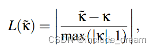
For curvatures, we compute the mean-square of the following rectified error for training and the RMS for evaluation. The rectified error L(k˜) is defined as:

在估计正态和真实正态之间。在训练期间，批处理上的均方欧几里德距离的性能略好，但为了更好的可解释性，我们使用均方根角度差来评估测试集上的结果。

对于曲率，我们计算以下修正误差的均方进行训练，并计算RMS（均方根角度差）进行评估。校正误差L(k ~)定义为:

Training and Evaluation Setup

Our network can be trained separately for normals and curvatures, or jointly to output both at the same time. In the joint network, the loss function is combined during training. We experiment with both variants to test whether the information about the curvatures can help normal estimation and vice versa, since the two are related. We train single-scale and multi-scale networks for each variant, each with 1024 point functions h.

The variants of our network are trained by selecting patches centered randomly at one of the 100K points in each point cloud. The radius of a patch is relative to the length of the bounding box of the point cloud. The single-scale networks are trained with a patch size of 0:05, and the multi-scale networks are trained with patch sizes of 0:01, 0:03, and 0:07. We use a fixed number of 500 points per patch. If there are fewer point within the patch radius, we pad with zeros (the patch center). The network can easily learn to ignore these padded points. If there are more points within the radius, we select a random subset. A more sophisticated subsampling method can be implemented in future work, which may be particularly beneficial for handling varying sampling densities.

In each epoch, we iterate through 1000 patches from each point cloud in the training set. We train for up to 2000 epochs on our dataset, or until convergence. Typically training converged before reaching this threshold, taking between 8 hours for single-scale architectures and 30 hours for multi-scale architectures on a single Titan X Pascal. A full randomization of the dataset, mixing patches of different shapes in each batch, was vital to achieve stable convergence. All our training was performed in PyTorch [pyt] using stochastic gradient descent with batch size 64, a learning rate of 10−4 and 0:9 momentum.

For evaluation, we select a random subset of 5000 points from each shape in the test set, and output the error of our method and the baseline methods over this subset. For the CGAL baseline methods [CGA], we use different patch sizes, where the size is determined by the number of nearest neighbors in the patch. For the small patch size we use the recommended setting of 18 nearest neighbors, and we increase the number of nearest neighbors by the same ratio as the area covered by our patches. This amounts to 112 and 450 nearest neighbors for the medium and large patches, respectively. For Boulch et al [BM16], we use the single-scale, 3scale and 5-scale networks provided by the authors.

训练和评估设置

**我们的网络可以分别训练法线和曲率，也可以联合训练法线和曲率同时输出。**在联合网络中，损失函数在训练过程中进行组合。我们对两种变量进行实验，以测试曲率信息是否有助于正态估计，反之亦然，因为两者是相关的。我们为每个变体训练单尺度和多尺度网络，每个变体都有1024个点函数h。

我们的网络变体是通过在每个点云的100K个点中选择随机中心的补丁来训练的。一个补丁的半径是相对于点云的边界框的长度。单尺度网络的patch大小为0:05，多尺度网络的patch大小为0:01、0:03和0:07。我们使用固定数量的500点每个补丁。如果patch半径内的点较少，则以0填充(patch中心)。网络可以很容易地学会忽略这些填充点。如果半径内有更多的点，我们选择一个随机子集。在未来的工作中可以实现更复杂的子采样方法，这可能特别有利于处理不同的采样密度。

在每个epoch中，我们从训练集中的每个点云迭代1000个补丁。我们在数据集上训练多达2000个epoch，或者直到收敛。通常，在达到这个阈值之前，训练是收敛的，在单个Titan X Pascal上，单尺度架构需要8小时，多尺度架构需要30小时。数据集的完全随机化，在每个批次中混合不同形状的补丁，对于实现稳定收敛至关重要。我们所有的训练都是在PyTorch [pyt]中进行的，使用随机梯度下降，批大小为64，学习率为10−4，动量为0:9。

为了评估，我们从测试集中的每个形状中选择5000个点的随机子集，并输出我们的方法和基线方法在该子集上的误差。对于CGAL基线方法[CGA]，我们使用不同的补丁大小，其中大小由补丁中最近邻居的数量决定。对于小的补丁大小，我们使用18个最近邻的推荐设置，并以与我们的补丁覆盖的面积相同的比例增加最近邻的数量。这相当于中型和大型斑块的最近邻分别为112和450个。对于Boulch等人[BM16]，我们使用作者提供的单尺度、3尺度和5尺度网络。

Result

Figure 3 shows the comparison of unoriented normal estimation using the methods discussed above. In this experiment, we consider either the output normal or the flipped normal, whichever has the lowest error. In the top section of the table, we show the results for varying levels of noise, from zero noise to high noise. The two rows in the middle show the results for point clouds with non-uniform sampling rate. In each of the categories we show the average for all 20 shapes in the category. The last row shows the global average error over all shapes. On the left, we show the level of error of each method in relation to the noise level of the input. The graph on the right shows the error of each method relative to the error of our single scale method (marked ss in the table).

We can observe the following general trends in these results: first, note that all of our methods consistently outperform competing techniques across all noise levels. In particular, observe that the methods based on jet fitting perform well under a specific intensity of noise, depending on the size of the neighborhood. For example, while jet small works well under small noise, it produces large errors strong noise levels. Conversely, jet large is fairly stable under strong noise but over-smooths for small noise levels, which leads to a large error for clean point clouds. One source of error of our current network compared, e.g. to the results of Boulch et al [BM16]

结果

图3显示了使用上述方法的无方向正态估计的比较。在这个实验中，我们考虑输出法线或翻转法线，以误差最小的为准。在表格的上半部分，我们显示了不同噪音水平的结果，从零噪音到高噪音。中间的两行是采样率不均匀的点云的结果。在每个类别中，我们显示了该类别中所有20个形状的平均值。最后一行显示了所有形状的全局平均误差。在左边，我们显示了每种方法的误差水平与输入噪声水平的关系。右图显示了每种方法相对于我们单比例尺方法的误差(表中标记为ss)。

我们可以在这些结果中观察到以下总体趋势:首先，请注意，我们所有的方法在所有噪声水平上都始终优于竞争技术。特别是，观察到基于射流拟合的方法在特定的噪声强度下表现良好，这取决于邻域的大小。例如，虽然射流小在小噪声下工作良好，但它会产生大的误差，强噪声水平。相反，射流大在强噪声下相当稳定，但在小噪声水平下过于平滑，这导致干净点云的误差很大。我们当前网络的一个误差来源，例如与Boulch等人[BM16]的结果进行了比较。

is that our method does not perform as well in the case of changes in sampling density. This is because our network was trained only on uniformly sampled point sets and therefore is not as robust to such changes. Nevertheless, it achieves comparable results across most levels of non-uniform sampling and shows significant improvement overall. For PointNet, we provide the performance on the training set in addition to the test set. PointNet overfits our training set, and the training set performance gives and approximate lower bound for the achievable error. Since PointNet’s point functions cover the whole point cloud, there is less resolution available for local details.

This results a large performance gap to other methods on detailed shapes, a gap that gets smaller with stronger noise, where the other methods start to miss details as well. Note also that our multi-scale architecture produces slightly better results than the single scale one for normal estimation. At the same time, the multi-scale architecture which combines both normals and curvature estimation (ms + c) produces slightly inferior results but has the advantage of outputting both normals and curvature at the same time.

我们的方法在抽样密度变化的情况下表现不佳。这是因为我们的网络只在均匀采样的点集上训练，因此对这种变化的鲁棒性不强。尽管如此，它在大多数非均匀抽样水平上取得了可比的结果，并显示出总体上的显着改进。对于PointNet，我们除了提供测试集之外，还提供了训练集上的性能。PointNet对训练集进行过拟合，训练集的性能给出了可达到误差的近似下界。由于PointNet的点函数覆盖了整个点云，因此局部细节的分辨率较低。

这导致与其他方法在细节形状上的性能差距很大，随着噪声的增强，差距会变小，而其他方法也会开始遗漏细节。还要注意的是，我们的多尺度体系结构比单尺度体系结构产生的正态估计结果稍好一些。同时，结合法线和曲率估计的多尺度架构(ms + c)的结果略差，但具有同时输出法线和曲率的优点。

（知识点补充：泊松重建
**泊松重建（Poisson Surface Reconstruction）是一种计算机图形学中的三维重建方法，用于从点云数据或深度图像生成平滑的三维曲面模型。**泊松重建的目标是通过点云数据或深度图像来还原连续的曲面，从而实现对物体或场景的三维形状的重建。

泊松重建的基本原理是利用泊松方程（Poisson Equation）来估计曲面的法向量，然后根据法向量生成平滑的曲面。具体来说，对于输入的点云数据或深度图像，首先计算其梯度或法向量信息。然后，利用泊松方程将法向量信息整合成一个连续的曲面。

泊松重建的优点在于生成的曲面平滑且无缝，能够有效地消除点云数据中的噪声和不完整性。此外，泊松重建还能够处理不规则的采样密度和边界条件，适用于从稀疏或噪声干扰较大的点云数据中还原出高质量的三维模型。

然而，泊松重建也有一些限制，例如对于边界不完整的点云数据可能会导致边界估计的不准确。因此，在应用泊松重建时，需要根据具体的数据情况选择合适的参数和预处理方法，以获得满足要求的三维重建结果。

知识点补充：泊松方程

泊松方程（Poisson Equation）是一个偏微分方程，广泛应用于数学、物理学和工程学等领域。在数学中，泊松方程描述了一个标量函数在空间中的分布和演化。

泊松方程通常可以表示为如下形式：

∇²u = f

其中，∇²u表示函数u的拉普拉斯算子，是函数u的各个偏导数的二阶混合导数之和。f是已知的标量函数，表示给定的边界条件或激励项。

泊松方程的解u是一个标量函数，它描述了在给定边界条件和激励项下，函数u在空间中的分布。在不同的领域中，泊松方程具有不同的解释和应用。在物理学中，泊松方程通常用于描述电势场、热传导等现象；在工程学中，它用于描述流体流动、结构力学等问题；在计算机图形学和计算机视觉中，泊松方程常用于图像处理、点云处理和图像重建等任务。

泊松方程的求解是一个重要的数值计算问题，常常通过数值方法，如有限差分法、有限元法或谱方法等来近似求解。这些数值方法能够有效地处理复杂的边界条件和几何形状，从而获得泊松方程的近似解，并在实际应用中发挥重要作用。
）

Poisson reconstruction from oriented normals estimated by PCPNET compared to baseline methods. Our method can reconstruct oriented normals with sufficient quality to successfully perform Poisson reconstruction, even in cases that are hard to handle by traditional methods. Although our method performs better on average, there are also failure cases, as demonstrated in the bottom row.

与基线方法比较，PCPNET估计的定向法向泊松重建。我们的方法可以在传统方法难以处理的情况下，以足够的质量重建定向法线，成功地进行泊松重建。尽管我们的方法在平均情况下表现得更好，但也有失败的情况，如下面一行所示。

is that our method does not perform as well in the case of changes in sampling density. This is because our network was trained only on uniformly sampled point sets and therefore is not as robust to such changes. Nevertheless, it achieves comparable results across most levels of non-uniform sampling and shows significant improvement overall. For PointNet, we provide the performance on the training set in addition to the test set. PointNet overfits our training set, and the training set performance gives and approximate lower bound for the achievable error. Since PointNet’s point functions cover the whole point cloud, there is less resolution available for local details.

This results a large performance gap to other methods on detailed shapes, a gap that gets smaller with stronger noise, where the other methods start to miss details as well. Note also that our multi-scale architecture produces slightly better results than the single scale one for normal estimation. At the same time, the multi-scale architecture which combines both normals and curvature estimation (ms + c) produces slightly inferior results but has the advantage of outputting both normals and curvature at the same time.

我们的方法在抽样密度变化的情况下表现不佳。这是因为我们的网络只在均匀采样的点集上训练，因此对这种变化的鲁棒性不强。尽管如此，它在大多数非均匀抽样水平上取得了可比的结果，并显示出总体上的显着改进。对于PointNet，我们除了提供测试集之外，还提供了训练集上的性能。PointNet对训练集进行过拟合，训练集的性能给出了可达到误差的近似下界。由于PointNet的点函数覆盖了整个点云，因此局部细节的分辨率较低。

这导致与其他方法在细节形状上的性能差距很大，随着噪声的增强，差距会变小，而其他方法也会开始遗漏细节。还要注意的是，我们的多尺度体系结构比单尺度体系结构产生的正态估计结果稍好一些。同时，结合法线和曲率估计的多尺度架构(ms + c)的结果略差，但具有同时输出法线和曲率的优点。

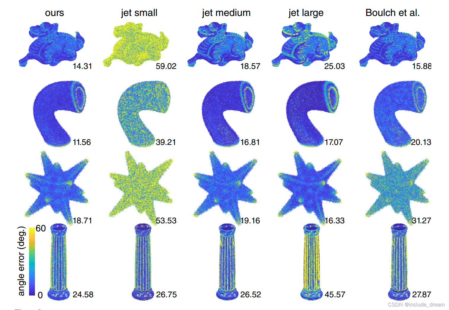
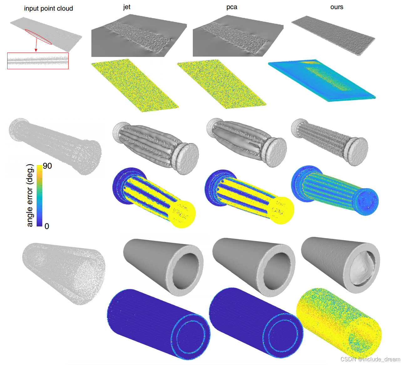
Qualitative comparison of the normals estimated by our method to the normals estimated by baseline methods. Shapes are colored according to normal angle error, where blue is no error and yellow is high error, numbers show the RMS error of the shape.

用我们的方法估计的正态线与基线方法估计的正态线的定性比较。形状根据法线角度误差着色，其中蓝色为无误差，黄色为高误差，数字表示形状的均方根误差。

In Figure 4 we show the results of the evaluation of our approach compared to baselines for oriented normal estimation. Namely, we use our pipeline directly for estimating oriented normals, and compare them to the jet fitting and PCA together with MST-based orientation propagation as implemented in CGAL [CGA]. We do not include the method of Boulch et al [BM16] in this comparison, as it is not designed to produce oriented normals. In Figure 4 we plot the RMS angle error while penalizing changes in orientation as well as the error relative to our performance. Finally, we also report the relative fraction of normals that are flipped with respect to the ground truth orientation, for other methods across different levels of noise.

Note that the errors in oriented normal estimation are highly correlated with the number of orientation flips, suggesting that the orientation propagation done during the post-processing is the main source of error. Also note that orientation propagation only works well for extremely small noise levels and very quickly deteriorates leading to large errors. Given a set of oriented normals, we can also perform Poisson reconstruction. Figure 8 shows a few examples of objects reconstructed with our oriented normals. Note that the topmost point cloud samples two sides of a thin sheet, making it hard to determine which side of the sheet a point originated from. In the middle row, the point cloud exhibits sharp edges that are hard to handle for the MST-based propagation. The bottom-most shape shows a failure case of our method. We suspect that a configuration like the inside of this pipe was not encountered during training. Increasing or diversifying the training set should solve this problem.

Note that on average, we expect the performance of our method for Poisson reconstruction to be proportional to the fraction of flipped normals, as shown in Figure 4.

Figure 7 shows the comparison of our curvature estimation to jet fitting. Due to the sensitivity of curvature to noise, noisy point clouds are a challenging domain for curvature estimation. Even though our method does not achieve a very high level of accuracy (recall that the error is normalized by the magnitude of the ground truth curvature), our performance is consistently superior to jet fitting on both principal curvature values, by a significant margin.

Qualitative comparisons of the normal error on four shapes of our dataset are shown in Figure 9. Note that for classical surface fitting (jet in these examples), small patch sizes work well on detailed structures like in the bottom row, but fail on noisy point clouds, while large patches are more tolerant to noise, but smooth out surface detail. Boulch et al [BM16] perform well in a low-noise setting, but the performance quickly degrades with stronger noise.

在图4中，我们显示了与面向正态估计的基线相比，我们的方法的评估结果。也就是说，我们直接使用我们的管道来估计定向法线，并将它们与射流拟合和PCA以及在CGAL [CGA]中实现的基于mst的定向传播进行比较。我们没有将Boulch等人[BM16]的方法包括在这个比较中，因为它不是设计用来产生定向法线的。在图4中，我们绘制了RMS角度误差，同时惩罚方向变化以及相对于我们的性能的误差。最后，我们还报告了相对于地面真值方向翻转的法线的相对比例，用于跨越不同噪声水平的其他方法。

请注意，定向正态估计的误差与方向翻转的次数高度相关，这表明在后处理期间进行的方向传播是误差的主要来源。还要注意的是，方向传播只适用于非常小的噪声水平，并且很快就会恶化，导致很大的误差。给定一组有向法线，我们也可以进行泊松重构。图8显示了用我们的定向法线重建的几个对象示例。请注意，最上面的点云采样薄板的两面，这使得很难确定一个点来自薄板的哪一面。在中间行，点云呈现出尖锐的边缘，这对于基于mst的传播来说是很难处理的。最底部的形状显示了我们方法的失败情况。我们怀疑在训练期间没有遇到像这个管道内部这样的配置。增加或多样化的训练集应该可以解决这个问题。

请注意，平均而言，我们期望泊松重建方法的性能与翻转法线的比例成正比，如图4所示。

图7显示了曲率估计与射流拟合的比较。由于曲率对噪声的敏感性，噪声点云是曲率估计的一个难点。尽管我们的方法没有达到非常高的精度水平(回想一下，误差是通过地面真实曲率的大小归一化的)，但我们的性能在两个主曲率值上始终优于喷气拟合，而且有很大的差距。

我们的数据集的四种形状的正态误差的定性比较如图9所示。请注意，对于经典的表面拟合(在这些例子中是jet)，小的补丁尺寸在像底部一行这样的细节结构上工作得很好，但在嘈杂的点云上就失败了，而大的补丁更能容忍噪音，但会使表面细节变得平滑。Boulch等[BM16]在低噪声环境下表现良好，但在强噪声环境下性能迅速下降。

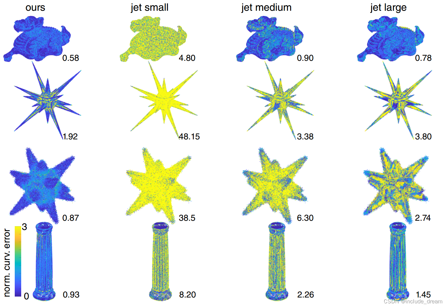
Qualitative comparison of curvature values estimated by our method to the curvature values estimated by a baseline method with three different patch sizes. Shapes are colored according to the curvature estimation error, where blue is no error and yellow is high error, numbers show the RMS error of the shape.

在三种不同的斑块大小下，我们的方法估计的曲率值与基线方法估计的曲率值的定性比较。形状根据曲率估计误差用颜色表示，其中蓝色表示无误差，黄色表示高误差，数字表示形状的均方根误差。

Even though our method does not always perform best in cases that are optimal for the parameter setting of a another method (e.g. versus jet fitting with large patch size in the third row, where the shape is very smooth and noisy), it performs better in most cases and on average.

In Figure 10, we show qualitative results of curvature estimation for selected shapes. The color of the points marks the error in curvature, where blue is no error and yellow is high error. Errors are computed in the same manner as described in Section 5.2, and are clamped between 0 and 3. The error of our curvature estimation is typically below 1, while for previous method the estimation is often orders of magnitude higher than the ground truth curvature.

尽管我们的方法在对另一种方法的参数设置最优的情况下并不总是表现最好(例如，与第三行具有大补丁尺寸的射流拟合相比，其中形状非常光滑和嘈杂)，但它在大多数情况下和平均情况下表现更好。

在图10中，我们展示了所选形状的曲率估计的定性结果。点的颜色表示曲率误差，其中蓝色表示没有误差，黄色表示高误差。误差的计算方法与第5.2节中描述的相同，并被限制在0和3之间。我们估计的曲率误差一般在1以下，而以前的方法估计的曲率往往比地面真曲率高几个数量级。

We presented a unified method for estimating oriented normals and principal curvature values in noisy point clouds. Our approach is based on a modification of a recently proposed PointNet architecture, in which we place special emphasis on extracting local properties of a patch around a given central point. We train the network on point clouds arising from triangle meshes corrupted by various levels of noise and show through extensive evaluation that our approach achieves state-of-the-art results across a wide variety of challenging scenarios. In particular, our method allows to replace the difficult and error-prone manual tuning of parameters, present in the majority of existing techniques with a data-driven training. Moreover, we show improvement with respect to other recently proposed learning-based methods.

While producing promising results in a variety of challenging scenarios, our method can still fail in some settings, such as in the presence of large flat areas, in which patch-based information is not enough to determine the normal orientation. For example, our oriented normal estimation procedure can produce inconsistent results, e.g., in the centers of faces a large cube. A more in-depth analysis and a better-adapted multi-resolution scheme might be necessary to alleviate such issues.

In the future, we also plan to extend our technique to estimate other differential quantities such as principal curvature directions or even the full first and second fundamental forms, as well as other mid-level features such as the Shape Diameter Function from a noisy incomplete point cloud. Finally, it would also be interesting to study the relation of our approach to graph-based neural networks [DBV16,HBL15] on graphs built from local neighborhoods of the point cloud.

提出了一种估计噪声点云中定向法线和主曲率值的统一方法。我们的方法是基于最近提出的PointNet架构的修改，其中我们特别强调提取给定中心点周围补丁的局部属性。我们在由各种程度的噪声损坏的三角形网格产生的点云上训练网络，并通过广泛的评估表明，我们的方法在各种具有挑战性的场景中取得了最先进的结果。特别是，我们的方法允许用数据驱动的训练取代大多数现有技术中存在的困难和容易出错的手动参数调优。此外，我们还展示了其他最近提出的基于学习的方法的改进。

虽然在各种具有挑战性的场景中产生了有希望的结果，但我们的方法仍然可能在某些设置中失败，例如在存在大片平坦区域的情况下，基于补丁的信息不足以确定正常方向。例如，我们的定向正态估计过程可能产生不一致的结果，例如，在面的中心有一个大立方体。可能需要更深入的分析和更适合的多分辨率方案来缓解这些问题。

在未来，我们还计划扩展我们的技术来估计其他微分量，如主曲率方向，甚至是完整的第一和第二基本形式，以及其他中级特征，如形状直径函数

一个嘈杂的不完全点云。最后，研究我们的方法与基于图的神经网络[DBV16,HBL15]在从点云的局部邻域构建的图上的关系也会很有趣。