Machine Learning - Logistic Regression - Two-class Classification

This series of articles are the study notes of " Machine Learning ", by Prof. Andrew Ng., Stanford University. This article is the notes of week 3, Logistic Regression part I. This article contains some topic about Logistic Regression, including classification, Decision boundary and Cost function.

Logistic Regression

1. Classification

In this and the next few sections, we'll start to talk about classification problems, where the variable y that you want to predict is valued. We'll develop an algorithm called logistic regression, which is one of the most popular and most widely used learning algorithms today. Here are some examples of classification problems.

Examples of Classification

Two-class (or binary) classification:

• Email: Spam / Not Spam?
• Online Transactions: Fraudulent (Yes / No)?
• Tumor: Malignant / Benign ? 

In all of these problems the variable that we're trying to predict is a variable y that we can think of as taking on two values either zero or one, either spam or not spam, fraudulent or not fraudulent, related malignant or benign. Another name for the class that we denote with zero is the negative class, and another name for the class that we denote with one is the positive class. So zero we denote as the benign tumor, and one, positive class we denote a malignant tumor. The assignment of the two classes, spam not spam and so on.

0: “Negative Class” (e.g., benign tumor)

1: “Positive Class” (e.g., malignant tumor) 

Multi-class classification:

How to develop a classification algorithm? 

Threshold classifier output h_θ(x) at 0.5: 

If you want to make predictions one thing you could try doing is then threshold the classifier outputs at 0.5 that is at a vertical axis value 0.5 and if the hypothesis outputs a value that is greater than equal to 0.5 you can take y = 1. If it's less than 0.5 you can take y=0.

• If  h_θ(x) ≥0.5, predict “y = 1”
• If  h_θ(x) <0.5, predict “y = 0” 

In this particular example, it looks like linear regression is actually doing something reasonable. Even though this is a classification toss we're interested in. But now let's try changing the problem a bit.

Add extra training example (on the right side)

Let me extend out the horizontal access a little bit and let's say we got one more training example way out there on the right. Notice that that additional training example, the one on the right, it doesn't actually change anything, right. Looking at the training set it's pretty clear what a good hypothesis is. Is that well everything to the right of somewhere around here, to the right of this we should predict this positive. Everything to the left we should probably predict as negative because from this training set, it looks like all the tumors larger than a certain value around here are malignant, and all the tumors smaller than that are not malignant, at least for this training set. But once we've added that extra example over here, if you now run linear regression, you instead get a straight line fit to the data. That might maybe look like the blue line. And if you know threshold hypothesis at 0.5, you end up with a threshold that's around here, so that everything to the right of this point you predict as positive and everything to the left of that point you predict as negative. And this seems a pretty bad thing for linear regression to have done.

linear regression to a classification problem often isn't a great idea

So, applying linear regression to a classification problem often isn't a great idea. In the first example, before I added this extra training example, previously linear regression was just getting lucky and it got us a hypothesis that worked well for that particular example, but usually applying linear regression to a data set, you might get lucky but often it isn't a good idea. So I wouldn't use linear regression for classification problems.

Here's one other funny thing about what would happen if we were to use linear regression for a classification problem. For classification we know that y is either zero or one. But if you are using linear regression where the hypothesis can output values that are much larger than one or less than zero, even if all of your training examples have labels y equals zero or one. And it seems kind of strange that even though we know that the labels should be zero.

Classification: y=1 or 0

But for linear regression: h_θ(x) can be >1 or <0

Logistic Regression is a classification algorithm

Logistic Regression: 0 ≤ h_θ(x) ≤ 1

The predictions of logistic regression are always between zero and one, and doesn't become bigger than one or become less than zero. And by the way, logistic regression is, and we will use it as a classification algorithm, is some, maybe sometimes confusing that the term regression appears in this name even though logistic regression is actually a classification algorithm.

2. Hypothesis representation

Let's start talking about logistic regression. In this section, I'd like to show you the hypothesis representation.

Logistic Regression Model 

That is, what is the function we're going to use to represent our hypothesis when we have a classification problem.We want 0 ≤h_θ(x) ≤ 1

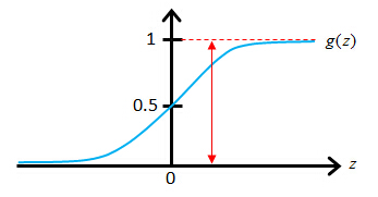
The sigmoid function g(z)

Sigmoid function also called Logistic function 

The sigmoid function, g(z), also called the logistic function, it looks like this. It starts off near 0 and then it rises until it crosses 0.5 and the origin, and then it flattens out again like so. So that's what the sigmoid function looks like. And you notice that the sigmoid function, while it asymptotes at one and asymptotes at zero, as a z axis, the horizontal axis is z. As z goes to minus infinity, g(z) approaches zero. And as g(z) approaches infinity, g(z) approaches one. And so because g(z) upwards values are between zero and one, we also have that h(x) must be between zero and one.

Interpretation of Hypothesis Output 

Here's how I'm going to interpret the output of my hypothesis, h_θ( x). When my hypothesis outputs some number, I am going to treat that number as the estimated probability that y is equal to one on a new input, example  x.

h_θ(x) = estimated probability that y = 1 on input x

Example:  

Let's say we're using the tumor classification example, so we may have a feature vector x, which is this x zero equals one as always. And then one feature is the size of the tumor. Suppose I have a patient come in and they have some tumor size and I feed their feature vector x into my hypothesis. And suppose my hypothesis outputs the number 0.7. I'm going to interpret my hypothesis as follows. I'm gonna say that this hypothesis is telling me that for a patient with features x, the probability that y equals 1 is 0.7. In other words, I'm going to tell my patient that the tumor, sadly, has a 70 percent chance, or a 0.7 chance of being malignant. 

If

Tell patient that 70% chance of tumor being malignant.

That means “ probability that y = 1, given x, parameterized by θ ” .

Now, since this is a classification task, we know that y must be either 0 or 1. Those are the only two values that y could possibly take on, either in the training set or for new patients that may walk into my office, or into the doctor's office in the future. So given h_θ( x), we can therefore

compute the probability that y = 0 as well, completely because y must be either 0 or 1.

So, you now know what the hypothesis representation is for logistic regression and we're seeing what the mathematical formula is, defining the hypothesis for logistic regression.

3. Decision boundary

What I'd like to do now is tell you about something called the  decision boundary, and this will give us a better sense of  what the logistic regressions hypothesis function is computing.

Logistic Regressions

To recap, this is what we wrote out last time, where we said that the hypothesis is represented as  h_θ(x)= g( θ ^Tx) equals g of theta transpose x, where g is this function called the sigmoid function, which looks like this. It slowly increases from zero to one, asymptoting at one. What I want to do now is

try to understand better when this hypothesis will make predictions that y is equal to 1 versus when it might make predictions that y is equal to 0. And understand better what hypothesis function looks like particularly when we have more than one feature.

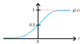
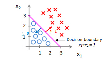
  Suppose predict “ y =1“  if  h_θ(x) ≥ 0.5

 predict “ y =0“  if  h_θ(x)< 0.5

Decision boundary

example 1

Predict "y=1", if  -3+x₁+x₂≥0,  that is, if  x₁+x₂≥3,  then "y=1"

Predict "y=0", if  -3+x₁+x₂<0,  that is, if  x₁+x₂<3,  then "y=0"

For any example which features   x ₁ and x ₂ that satisfy this equation, that minus 3 plus   x ₁+ x ₂ is greater than or equal to 0, our hypothesis will think that y equals 1, the small x will predict that y is equal to 1. We can also take -3 and bring this to the right and rewrite this as   x ₁+ x ₂ is greater than or equal to 3, so equivalently, we found that this hypothesis would predict y=1 whenever  x ₁+ x ₂ is greater than or equal to 3.

example 2 

Earlier when we were talking about polynomial regression or when we're talking about linear regression, we talked about how we could add extra higher order polynomial terms to the features. And we can do the same for logistic regression. Concretely, let's say my hypothesis looks like this where I've added two extra features, x ₁ ² and x ₂ ², to my features. So that I now have five parameters, θ ₀ through θ ₄.

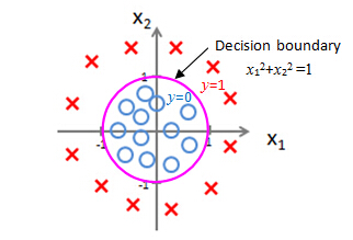
Predict "y=1", if  -1+x₁²+x₂²≥0,  that is, if x₁²+x₂²≥1,  then "y=1"

Predict "y=0", if  -1+x₁²+x₂²<0,  that is, if x₁²+x₂²<1,  then "y=0"

If we plot the curve for x₁²+x₂²=1, you will recognize that, that is the equation for circle of radius one, centered around the origin. So that is my decision boundary. And everything outside the circle, I'm going to predict as y=1. So out here is my y=1 region, we'll predict y=1 out here and inside the circle is where I'll predict y=0.

So by adding these more complex, or these polynomial terms to my features as well, I can get more complex decision boundaries that don't just try to separate the positive and negative examples in a straight line that I can get in this example, a decision boundary that's a circle. 

The decision boundary is a property of the hypothesis under the parameters

The decision boundary is a property, not of the trading set, but of the hypothesis under the parameters. So, so long as we're given my parameter vector theta, that defines the decision boundary, which is the circle. But the training set is not what we use to define the decision boundary. The training set may be used to fit the parameters theta. We'll talk about how to do that later. But, once you have the parameters theta, that is what defines the decisions boundary.

4. Cost function

In this section, we'll talk about how to fit the parameters of theta for the logistic compression. In particular, I'd like to define the optimization objective, or the cost function that we'll use to fit the parameters. Here's the supervised learning problem of fitting logistic regression model.

Logistic Regression Model

We have a training set of m training examples and as usual, each of our examples is represented by a that's n plus one dimensional, and as usual we have x o equals one. First feature or a zero feature is always equal to one. And because this is a computation problem, our training set has the property that every label y is either 0 or 1. This is a hypothesis, and the parameters of a hypothesis is this theta over here. And the question that I want to talk about is given this training set, how do we choose, or how do we fit the parameter's θ?

Training set: m examples

Hypothesis

How to choose parameters θ?

Cost Function

Back when we were developing the linear regression model, we used the following cost function. I've written this slightly differently where instead of 1/2 m, I've taken a one-half and put it inside the summation instead. Now I want to use an alternative way of writing out this cost function. 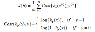Which is that instead of writing out this square of return here, let's write in here costs of   h_θ( x), y and I'm going to define that total cost of   h_θ( x), y to be equal to this. Just equal to this one-half of the squared error. So now we can see more clearly that the cost function is a sum over my training set, which is 1 over n times the sum of my training set of this cost term here. And to simplify this equation a little bit more, it's going to be convenient to get rid of those superscripts. So just define cost of   h_θ( x) comma y to be equal to one half of this squared error. And interpretation of this cost function is that, this is the cost I want my learning algorithm to have to pay if it outputs that value, if its prediction is   h_θ( x), and the actual label was y.

Linear Regression

So, the cost function of a single example x can be written as

This cost function worked fine for linear regression. But it turns out that if we use this particular cost function in logistic regression, this would be a non-convex function of the parameter's data. Here's what I mean by non-convex. Have some cross function J(θ) and for logistic regression, this function h here has a nonlinearity that is one over one plus e to the negative theta transpose. So this is a pretty complicated nonlinear function.If you want to make predictions one thing you could try doing is then threshold the classifier outputs at 0.5 that is at a vertical axis value 0.5 and if the hypothesis outputs a value that is greater than equal to 0.5 you can take y = 1. If it's less than 0.5 you can take y=0.

non-convex function

You find that J( θ) can look like a function that's like the left curve with many local optima. And this is a non-convex function. If you run gradient descent on this sort of function,  it is not guaranteed to converge to the global minimum. 

convex function

Whereas in contrast what we would like is to have a cost function J(θ) that is convex, that is a single bow-shaped function that looks like the right side curve so that if you run gradient descent on this sort of function, we would be guaranteed that would converge to the global minimum.

Logistic Regression Cost Function of Single Example

So what we'd like to do is, instead of come up with a different cost function, that is convex, and so that we can apply a great algorithm, like gradient descent and be guaranteed to find the global minimum. Here's the cost function that we're going to use for logistic regression.

This is the cost function with a single example x

Here is the plot of y= log(z).

So, we can draw the cost function below when y=1.

First, if y=1 and h_θ(x)=1,in other words, if the hypothesis exactly predicts h_θ(x)=1 and y is exactly equal to what it predicted, then the cost = 0. And that's where we'd like it to be because if we correctly predict the output y,then the cost is 0.

But now notice also that as h_θ( x) approaches 0, so as the output of a hypothesis approaches 0, the cost blows up and it goes to infinity. And what this does is this captures the intuition that if a hypothesis of 0, that's like saying a hypothesis saying the chance of y equals 1 is equal to 0.

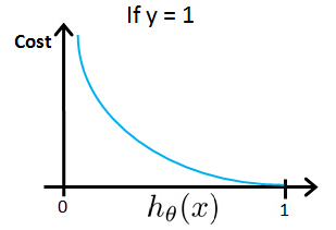
Cost = 0, if y =1 ,h_θ(x) = 1

But as  h_θ(x) → 0,  Cost → ∞

Captures intuition that if h_θ(x)=0,(predict P(y=1|x;θ)=0), but y=1, we'll penalize learning algorithm by a very large cost.

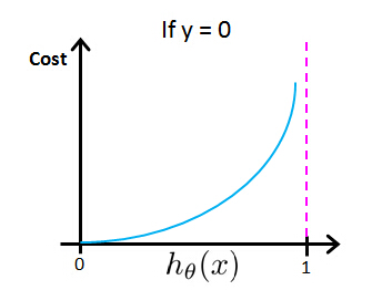
Cost = 0, if y =0 ,h_θ(x) = 0

But as  h_θ(x) → 1,  Cost → ∞

So if y=0, that's going to be our cost function, if you look at this expression and you plot -log(1-z), if you figure out what that looks like, you get a figure that looks like this which goes from 0 to a with the z axis on the horizontal axis. So if you take this cost function and plot it for the case of y=0, what you get is that the cost function. Looks like the curve above. And, what this cost function does is that it goes up or it goes to a positive infinity as h of x goes to 1, and this catches the intuition that if a hypothesis predicted that your h of x is equal to 1 with certainty, with probably ones, absolutely going to bey=1.But if y turns out to be equal to 0, then it makes sense to make the hypothesis. So the make the learning algorithm up here a very large cost. And conversely, if h_θ(x) =0 and y=0, then the hypothesis melted. The protected y of z is equal to 0, and it turns out y is equal to 0, so at this point, the cost function is going to be 0.

In this section, we define the cost function for a single train example. The topic of convexity analysis is now beyond the scope of this course, but it is possible to show that with a particular choice of cost function, this will give a convex optimization problem. Overall cost function J(θ) will be convex and local optima free. 

5. Simplified cost function and gradient descent

Logistic Regression Cost Function

Note, y=1 or y=0 always, so

The cost function can be written as,

To fit parameters θ

Given this cost function J(θ), in order to fit the parameters, what we're going to do then is try to find the parametersθ that minimize J(θ). So if we try to minimize this, this would give us some set of parametersθ. 

Finally, if we're given a new example with some set of features x, we can then take the thetas that we fit to our training set and output our prediction as this.

To make a prediction given new x, output

And just to remind you, the output of my hypothesis I'm going to interpret as the probability that y is equal to one. And given the input x and parameterized by theta: P(y=1|x; θ). But just, you can think of this as just my hypothesis as estimating the probability that y is equal to one.

Gradient Descent 

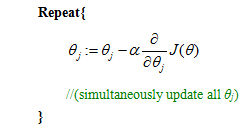
Want min_θ J(θ):

If we compute the partial derivative term in the update equation above,

So if you take this partial derivative term and plug it back in here, we can then write out our gradient descent algorithm as follows. 

So if you have n features, you would have a parameter vector theta, which with parameters theta 0, theta 1, theta 2, down to theta n. And you will use this update to simultaneously update all of your values of theta. Now, if you take this update rule and compare it to what we were doing for linear regression. You might be surprised to realize that, well, this equation was exactly what we had for linear regression. In fact, if you look at the earlier videos, and look at the update rule, the Gradient Descent rule for linear regression. It looked exactly like what I drew here inside the blue box. So are linear regression and logistic regression different algorithms or not? Well, this is resolved by observing that for logistic regression, what has changed is that the definition for this hypothesis has changed. This is actually not the same thing as gradient descent for linear regression.

In Linear Regression:

In Logistic Regression:

Make sure your gradient descent work correctly

In an earlier video, when we were talking about gradient descent for linear regression, we had talked about how to monitor a gradient descent to make sure that it is converging. I usually apply that same method to logistic regression, too to monitor a gradient descent, to make sure it's converging correctly. And hopefully, you can figure out how to apply that technique to logistic regression yourself. 

Plot

as a function of the number of iterations and make sure J(θ) is decreasing on every iteration.

When implementing logistic regression with gradient descent, we have all of these different parameter values, theta zero down to theta n, that we need to update using this expression. And one thing we could do is have a for loop. So for i equals zero to n, or for i equals one to n plus one. So update each of these parameter values in turn. But of course rather than using a for loop, ideally we would also use a vector rise implementation. So that a vector rise implementation can update all of these m plus one parameters all in one fell swoop. And to check your own understanding, you might see if you can figure out how to do the vector rise implementation with this algorithm as well. 

Feature Scaling

Now you know how to implement gradient descents for logistic regression. There was one last idea that we had talked about earlier, for linear regression, which was feature scaling. We saw how feature scaling can help gradient descent converge faster for linear regression. The idea of feature scaling also applies to gradient descent for logistic regression. And yet we have features that are on very different scale, then applying feature scaling can also make grading descent run faster for logistic regression. So that's it, you now know how to implement logistic regression and this is a very powerful, and probably the most widely used, classification algorithm in the world. And you now know how we get it to work for yourself.