PRML 1 INTRODUCTION

PRML is one of classical book about pr and ml. 

1 Introduction

The training data set : a large set of N digits{x1, x2, x3, ... xN}, the training vector x. we use it to tune the parameters of an adaptive model. 

sometimes, we have an corresponding digit {t1, t2, t3, ... tN}, the target vector t (supervised learning problems). 

The goal of ML is finding an optimal function y(x) between the  training data and target vector t.（隐藏在data背后的规律）

we use a function y(x) which takes the training vector x as an input and generates an output (the target vector t). after training the model, we get the function y(x), then we can predict corresponding output for a new vector x.

2 Pre-processing can speed up the computation by feature extraction. we use feature vector, maybe not all of the training data. care must be taken during pre-processing cause often the information is discarded.

3 This is known as an supervised learning problems (we have an target vector t), which conclude regression and classification e.t. unsupervised problem conclude clustering, density estimation.  

4 The distance between regression and classification: for regression problems, the target vector t will comprise continuous variables, for classification problems, t will represent class labels and comprise discrete variables.

5 reinforcement learning. ...

6 an interesting example: Polynomial Carve Fitting: Our goal is to exploit this training set in order to make predictions of the value of target variable t under some new value of input variable x.

a training data: X={x1, x2, ... xN}, and the corresponding observation: T={t1, t2, ... tN};

this data is generalized by function , we use the training data and target data to learn an polynomial y(x,w), which was approach their relationship  .(ML的目的是对于新的数据，预测对应的值，例如房子的面积和价格，通过训练样本X，采用多项式拟合，可以学习到隐藏在数据中的关系y(x,w)=(w)T*x,对于新的数据h，return (w)T*h,称之为回归regression)。

.

对于w，有很多种选择，

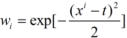
当你的训练数据x(i)与观测数据很近时，wi=1，当训练数据与观测数据很远时，wi=1；在这种选择下，系数w其实是[0,1]，意味着会自动保留那些比较近的数据，而抛弃远的数据。

after model this relationship, how to make sure the coefficient  w. the values of the coefficients will be determined by fitting the polynomial to the training data. This can be done by minimizing the error function.One of the simple choice is given by the sum of squares of the errors between the predictions y(x;w) of training data x and corresponding target values t.

7 Over-fitting

{1 there must be noise mixture in the training data, and we design an model with it; 

2 there may be some data belongs to other models, so we design an suitable model which we want to.}

{1 increase the size of training set;

2  regularization (for minimize squares error);

3 design other models(for example, adopt a Bayesian approach).

}

We may find an vector w, which make the error function E(w)=0；but the fitted curve was badly represented of the function .

M is the order of coefficient w.（控制单个模型的复杂度）

If M is too small, then the polynomial fit the curve poor(poor-fitting); 

If M is big, may the error function is equal to 0, on the contrast the polynomial gives a very poor representation of the function  too(over-fitting).

 one technique that is often used to control the over-fitting phenomenon is regularization, which involves adding a penalty term to the error function E(W).

（w控制着model的复杂度，overfitting的原因1训练样本太少，2模型过于复杂，3data中含有噪声。）

Technique such as regularization are known in the statistics literature as shrinkage methods.

8 we can express our uncertainty over the value of the target variable using a probability distribution and assume all the data has a Gaussian distribution and are i.i.d, then we have 

then use maximum likelihood, we got 

9 Bayesian curve fitting

Bayes' theorem in words 

we use the prior distribution and the likelihood function to get the posterior distribution

and Maximum the posterior probability(MAP)

最大化似然函数对应于一般的最小二乘法，而最大化后验概率对应于正则化的二乘。

10Decision Theory

Bayesian decision 是解决模式识别问题的一种基本的方法，几乎所有的书都会讲Bayesian。目的是给定new value x，确定最优的输出t。

基本思想如下：

★已知类条件概率密度参数表达式和先验概率；
★利用贝叶斯公式转换成后验概率；
★根据后验概率大小进行决策（regression和classification）。

generative model 

同时对输入和输出建模，对于一个训练样本x，对应于一个类别CK，

generative model对每一对数据进行建模p(x|ck)；在计算p(ck);

p(x)=求和{p(x|ck)p(ck)};

p(ck|x)={p(x|ck)p(ck)}/p(x);

通过观测数据，计算p(x|ck)和p(ck)，去计算p(ck|x)。

贝叶斯估计中，假设参数是确定的随机变量，服从一定的分布，选择model（即选择参数服从的分布-概率密度函数），例如：Bernoulli distribution 与 Beta distribution，Gaussian distribution 与 Gaussian distribution，Multinomial distribution 与Dirichlet distribution。
贝叶斯估计中一般假设样本是独立同分布（i.i.d）。
Bayesian estimation的步骤：
(1)确定参数的先验分布；
(2)由样本的概率分布（是参数的概率密度函数，还是data的概率分布？这个地方有些模糊），计算类条件概率分布（即似然函数）；并根据Bayesian法则计算后验概率分布—Bayesian估计中，参数的概率密度函数（样本的概率密度函数还是参数的）；
共轭先验是为了计算后验概率分布时，先验概率分布和类条件概率分布具有相同的形式，从大大的简化计算。
(3)计算出参数的Bayesian估计值。例如根据概率密度函数，计算参数的期望和方差等。

预测分布的积分式中，一个是参数的后验概率分布，另一个是类条件概率分布，似然函数？这个积分表达的意义，不是很理解，只是知道利用共轭分布的性质，计算后得到的是对于新的样本值x，所对应的目标值t的分布概率密度，即与新的输入x相对应的输出t的分布，是一种预测，预测的分布概率密度。

discriminative model 

直接对p(ck|x)进行建模。即直接计算p(ck|x)。