SVM代码实现（硬间隔+软间隔）

目录

1、线性可分支持向量机/硬间隔支持向量机
适用场景：训练数据线性可分
方法：通过硬间隔最大化
2、线性支持向量机/软间隔支持向量机
适用场景：训练数据近似线性可分
方法：通过软间隔最大化
3、代码
1）线性可分支持向量机的实现
2）线性支持向量机的实现以及五折交叉验证进行寻找最佳的惩罚系数C

1、线性可分支持向量机/硬间隔支持向量机

数据集：T={（x1,y1），（x2,y2），…，（xN,yN）}
(xi，yi)为一个训练样本，xi为一个实例，yi为该实例的分类。yi为1时为正例，yi为-1时为负例。
学习目标：在特征空间寻找一个分离超平面（将两类正确分类并且使得两类几何间隔最大）：wx+b=0，该超平面由法向量w和截距b决定。法向量指向的一侧为正类。
相应的分类决策函数：f(x)=sign(wx+b) 称为线性可分支持向量机

间隔
函数间隔：
y(wx+b)表示分类的正确性以及确信度
（正确性：是否分类正确 y和wx+b是否同号来确定）
（确信度：|wx+b|表示当wx+b=0确定时，样本点距离超平面的远近）
超平面（w,b）关于样本点（xi,yi）的函数间隔：
ri’=yi(wxi+b)
超平面（w,b）关于数据集T的函数间隔（所有样本点中函数间隔最小值）：
r‘=min(ri)=min(yi(w*xi+b))
几何间隔

超平面（w,b）关于样本点（xi,yi）的几何间隔：
ri=yi(wxi+b)//||w||
超平面（w,b）关于数据集T的几何间隔（所有样本点中几何间隔最小值）：
r=min(ri)=min(yi(wxi+b))/||w||
ps：若w、b成比例的变化，即超平面不改变，此时函数间隔也会成比例变化，而几何间隔不变。

优化问题

1、希望数据集几何间隔最大，并且每一个样本点均大于这个间隔

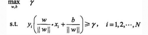
2、根据几何间隔和函数间隔的联系：

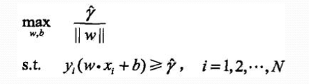
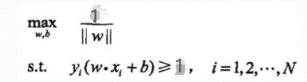
3、我们知道同比例改变w、b，函数间隔会同比例变化，故

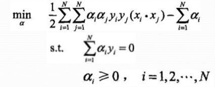
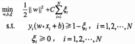
4、变求最大为求最小，则

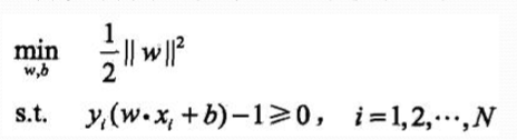
该问题是一个凸优化问题，凸优化问题定义如下：

通常转换为拉格朗日对偶问题来求解
5、学习的对偶算法

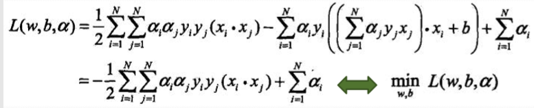
a的求解方法：

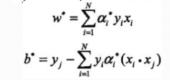
w、b的求解方法：

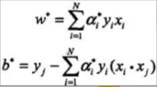
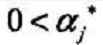
其中a的取值范围是

2、线性支持向量机/软间隔支持向量机

当数据中有一些奇异点，如下图中跑上来的两个红色的点。只是这极个别的点而导致的非完全线性可分。 此时，需要对每个样本点增加一个松弛变量。

这样该问题的原始问题就变成了

与线性可分支持向量机同样的分析过程，其对偶问题变为了
（a求解方法）

（w b求解方法）

其中 a的取值范围为

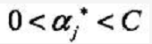
（具体原因分析KKT条件）

3、代码

重点问题：
1）因两个问题均为凸优化问题，使用cvxopt库中的solvers.qp方法进行求解a，分析其中参数得（如何寻找的大家可以对照着qp问题格式依次对应即可）：
（推荐一个相关的博客，简单的举了个例子https://www.jianshu.com/p/df447c3e4efe）
求解线性可分支持向量机对应的参数

求解线性支持向量机对应的参数

2）对应线性支持向量机五折交叉验证寻找最优的C。
设置C 的范围为[1e-3,1e-2,1e-1,1,1e1,1e2,1e3]、交叉验证折数5，进行双重循环（循环C和5）执行线性支持向量机算法，对于每一个C求一次平均正确率，最终根据最高的正确率选择最优的C，再投入到线性支持向量算法中。

3）涉及到numpy和cvxopt中一些简单函数
放到另外一篇博客中
链接：https://blog.csdn.net/jichun4686/article/details/102948023

（ 代码参考：https://www.cnblogs.com/buzhizhitong/p/6089070.html
https://blog.csdn.net/huakai16/article/details/78070671 整体思想相同，仅加入了我自己的理解）

代码主体如下：

import numpy as np
import matplotlib.pyplot as plt
from cvxopt import solvers
import cvxopt

def linear_kernel(x1,x2):
    return np.dot(x1,x2)

class mySVM():
    def __init__(self,kernel=linear_kernel,C=None):
        self.kernel = kernel     #这是一个函数  代指其核的运算
        self.C = C
    def fit(self,X,y):
        n_samples = X.shape[0]
        n_feature = X.shape[1]

        #求凸优化问题需要的参数  P q G h A b
        #先求x的核矩阵  以方便求P
        K = np.zeros((n_samples,n_samples))
        for i in range(n_samples):
            for j in range(n_samples):
                K[i][j] = self.kernel(X[i],X[j])
        P = cvxopt.matrix(np.outer(y,y)*K)
        q = cvxopt.matrix(np.ones(n_samples) * -1)   #为列向量  √
        A = cvxopt.matrix(y,(1,n_samples))    #y的转置 为行向量   （1，n_samples）表示排列为1*n_samples的矩阵
        b = cvxopt.matrix(0.0)

        #对于线性可分数据集
        if self.C is None:
            G = cvxopt.matrix(np.diag(np.ones(n_samples) * -1))
            h = cvxopt.matrix(np.zeros(n_samples))
        #对于软间隔
        else:
            arg1 = np.diag(np.ones(n_samples) * -1)
            arg2 = np.diag(np.ones(n_samples))
            G = cvxopt.matrix(np.vstack((arg1,arg2)))   #加括号  因为vstack只需要一个参数
            arg1 = np.zeros(n_samples)
            arg2 = np.ones(n_samples) * self.C
            h = cvxopt.matrix(np.hstack((arg1,arg2)))

        solution  = solvers.qp(P,q,G,h,A,b)

        a = np.ravel(solution['x'])

        if self.C is None:
            sv = a>1e-5
        else:
            sv = (a > 1e-5) * (a < self.C)

        index = np.arange(len(a))[sv]   #a>1e-5  返回true or false的数组   取出对应为true的下标

        self.a = a[sv]  #大于0对应的a的值index
        self.sv_X = X[sv]  #支持向量的X index
        self.sv_y = y[sv]    #支持向量的y  index

        print('%d 点中有 %d 个支持向量' %( n_samples,len(self.a)))

        ###算 w  以及  b
        #求w
        self.w = np.zeros(n_feature)
        for i in range(len(self.a)):
            self.w += self.a[i] * self.sv_y[i] * self.sv_X[i]
        # print(self.w)
        #求b
        self.b = 0
        for i in range(len(self.a)):
            self.b += self.sv_y[i]
            self.b -= np.sum(self.a * self.sv_y * K[index[i]][index])
        self.b /= len(self.a)
        # print(self.b)

    def predict(self,X_test):
        return np.sign(np.dot(X_test,self.w) + self.b)   #注意X_text  self.w不要写反

    def plot(self,X1_train,X2_train):
        def f(x,w,b,c):
            #w0*x0 + w1*x1 +b =c
            return  (-w[0] * x - b + c)/w[1]

        plt.scatter(self.sv_X[:, 0], self.sv_X[:, 1], color='black', s=100)
        plt.scatter(X1_train[:,0],X1_train[:,1],color='blue',label='1')
        plt.scatter(X2_train[:,0],X2_train[:,1],color='red',label='-1')

        #wx + b = 0    w0*x0 + w1*x1 +b =0
        x0_1 = 4
        y0_1 = f(x0_1,self.w,self.b,0)
        x0_2 = -3
        y0_2 = f(x0_2,self.w,self.b,0)
        plt.plot([x0_2,x0_1],[y0_2,y0_1],'k')

        #wx + b = 1    w0*x0 + w1*x1 +b = 1
        x1_1 = 4
        y1_1 = f(x1_1,self.w,self.b,1)
        x1_2 = -3
        y1_2 = f(x1_2,self.w,self.b,1)
        plt.plot([x1_2,x1_1],[y1_2,y1_1],'k--')

        #wx + b = -1   w0*x0 + w1*x1 +b = -1
        x2_1 = 4
        y2_1 = f(x2_1,self.w,self.b,-1)
        x2_2 = -3
        y2_2 = f(x2_2,self.w,self.b,-1)
        plt.plot([x2_2,x2_1],[y2_2,y2_1],'k--')

        plt.xlabel('x')
        plt.ylabel('y')
        plt.show()
        plt.close()


def dataSelection(type):
 
    #随机产生的数据
    #随机产生的线性可分数据
    mean1_1 = np.array([0, 2])
    mean2_1 = np.array([2, 0])
    cov_1 = np.array([[0.8, 0.6], [0.6, 0.8]])
    X1_1 = np.random.multivariate_normal(mean1_1, cov_1, 100)
    y1_1 = np.ones(len(X1_1))   #行向量
    X2_1 = np.random.multivariate_normal(mean2_1, cov_1, 100)
    y2_1 = np.ones(len(X2_1)) * -1

    #随机产生的线性可分但是有部分重叠的数据
    mean1_2 = np.array([0, 2])
    mean2_2 = np.array([2, 0])
    cov_2 = np.array([[1.7, 1.0], [1.0, 1.7]])  #原来
    # cov_2 = np.array([[1, 0.5], [0.5, 1]])
    X1_2 = np.random.multivariate_normal(mean1_2, cov_2, 100)
    y1_2 = np.ones(len(X1_2))
    X2_2 = np.random.multivariate_normal(mean2_2, cov_2, 100)
    y2_2 = np.ones(len(X2_2)) * -1
    #随机产生线性不可分的数据
    mean1_3 = [-1, 2]
    mean2_3 = [1, -1]
    mean3_3 = [4, -4]
    mean4_3 = [-4, 4]
    cov_3 = [[1.0, 0.8], [0.8, 1.0]]
    X1_3 = np.random.multivariate_normal(mean1_3, cov_3, 50)
    X1_3 = np.vstack((X1_3, np.random.multivariate_normal(mean3_3, cov_3, 50)))
    y1_3 = np.ones(len(X1_3))
    X2_3 = np.random.multivariate_normal(mean2_3, cov_3, 50)
    X2_3 = np.vstack((X2_3, np.random.multivariate_normal(mean4_3, cov_3, 50)))
    y2_3 = np.ones(len(X2_3)) * -1

    if  type=='random_linear':
        return X1_1, y1_1, X2_1, y2_1
    elif type == 'random_linear_soft':
        return X1_2, y1_2, X2_2, y2_2
    elif type == 'random_nonlinear':
        return X1_3, y1_3, X2_3, y2_3

#划分数据集测试集
def split_train_test(X1,Y1,X2,Y2,ratio):
    samples_num = len(Y1)
    num_train = int(samples_num * ratio)
    # num_test = samples_num * (1-ratio)

    X1_train = X1[:num_train]
    Y1_train = Y1[:num_train]
    X2_train = X2[:num_train]
    Y2_train = Y2[:num_train]
    X_train = np.vstack((X1_train,X2_train))  ###需要加两个括号
    y_train = np.append(Y1_train,Y2_train)    #用hstack也可以

    X1_test = X1[num_train:]
    Y1_test = Y1[num_train:]
    X2_test = X2[num_train:]
    Y2_test = Y2[num_train:]
    X_test = np.vstack((X1_test,X2_test))
    y_test = np.append(Y1_test,Y2_test)


    return X_train,y_train,X_test,y_test

def test_randomLinear():
    X1, y1, X2, y2 = dataSelection('random_linear')
    X_train, y_train, X_test, y_test=split_train_test(X1, y1, X2, y2, 0.9)

    clf = mySVM()
    clf.fit(X_train,y_train)

    y_predict = clf.predict(X_test)
    correct = np.sum(y_predict == y_test)
    print("%d 个测试样本中有%dg个预测正确" % (len(y_predict),correct))
    clf.plot(X_train[y_train==1],X_train[y_train==-1])

def test_randomLinearSoft():

    # X1, y1, X2, y2 = dataSelection('iris_linear')
    X1, y1, X2, y2 = dataSelection('random_linear_soft')
    X_train, y_train, X_test, y_test=split_train_test(X1, y1, X2, y2, 0.9)

    clf = mySVM(C=10)
    clf.fit(X_train,y_train)

    y_predict = clf.predict(X_test)
    correct = np.sum(y_predict == y_test)
    print("%d 个测试样本中有%dg个预测正确" % (len(y_predict),correct))
    clf.plot(X_train[y_train==1],X_train[y_train==-1])


def find_bestC(X1, y1, X2, y2):
    folds = 5
    cs = [-3,-2,-1,0,1,2,3]
    Cs = []
    for c in cs:
        Cs.append(np.power(10.,c))
    # Cs = [1e-3,1e-2,1e-1,1,1e1,1e2,1e3]

    # X1, y1, X2, y2 = dataSelection('random_linear_soft')
    X1_folds = np.vsplit(X1,folds)
    X2_folds = np.vsplit(X2,folds)
    y1_folds = np.hsplit(y1,folds)
    y2_folds = np.hsplit(y2,folds)

    accuracy_of_C = {}  #字典类型

    for C in Cs:
        accuracy_of_C[C] = []
        for i in range(folds):   #fold 0 1 2 3 4
            temp1 = np.vstack(X1_folds[:i]+X1_folds[i+1:])
            temp2 = np.vstack(X2_folds[:i]+X2_folds[i+1:])
            X_train = np.vstack((temp1,temp2))

            temp1 = np.hstack(y1_folds[:i]+y1_folds[i+1:])
            temp2 = np.hstack(y2_folds[:i]+y2_folds[i+1:])

            y_train = np.hstack((temp1,temp2))
            X_test = np.vstack((X1_folds[i],X2_folds[i]))
            y_test = np.hstack((y1_folds[i],y2_folds[i]))

            clf = mySVM(C=C)
            clf.fit(X_train,y_train)
            y_predict = clf.predict(X_test)
            correct = np.sum(y_predict == y_test)
            accuracy = float(correct)/len(y_test)
            accuracy_of_C[C].append(accuracy)
            print("当C为%f 时 第 %d 组 %d 个测试样本中有%dg个预测正确" % (C,i,len(y_predict),correct))
    accuracys = []
    for C in Cs:
        avgacc = 0.0
        for accuracy in accuracy_of_C[C]:
            avgacc += accuracy
            print('C = %f,accuracy = %f' %(C,accuracy))
        temp = avgacc/len(accuracy_of_C[C])
        accuracys.append(temp)
    ##求np数组的最大值的下标 np.arg(xx)  求列表最大值的下标xx.index(max(xx))
    bestC_index = accuracys.index(max(accuracys))
    bestC = Cs[bestC_index]
    print(bestC)

    plt.plot(cs,accuracys)

    plt.show()
    plt.close()

    return bestC
    # print(accuracys)

def test_randomLinearSoft2():
    X1, y1, X2, y2 = dataSelection('random_linear_soft')
    X_train, y_train, X_test, y_test = split_train_test(X1, y1, X2, y2, 0.9)

    bestC = find_bestC( X1, y1, X2, y2)

    clf = mySVM(C=bestC)
    clf.fit(X_train,y_train)

    y_predict = clf.predict(X_test)
    correct = np.sum(y_predict == y_test)
    print("%d 个测试样本中有%dg个预测正确" % (len(y_predict),correct))
    clf.plot(X_train[y_train==1],X_train[y_train==-1])

def draw(datas):
        plt.scatter(datas[:50,0],datas[:50,1],color='blue',label='1(iris +)')
        plt.scatter(datas[50:,0],datas[50:,1],color='red',label='-1(iris -)')
        plt.xlabel('SepalLengthCm')
        plt.ylabel('SepalWidthCm')
        plt.legend(loc='upper Data')  #标签位置  左上角
        plt.title('SVM_withoutC')

        # x1 = 4.0
        # y1 = -((self.weights[0]*x1+self.bias)/(self.weights[1]))
        # x2 = 7.0
        # y2 = -((self.weights[0] * x2 + self.bias) / (self.weights[1]))
        # plt.plot([x1, x2], [y1, y2], 'yellow')

        plt.show()
        plt.close()



if __name__ == '__main__':
    # dataslinear = dataSelection('linear')
    # print(dataslinear)
    # draw(dataslinear)
    # test_randomLinear()
    # test_randomLinearSoft() #指定惩罚系数
    test_randomLinearSoft2()  #五折交叉验证来求得最好的C后放入SVM软间隔支持向量机
    # find_bestC()   #五折交叉验证来求得最好的C 

如有问题，请多多指正。