


需要源码和数据集请点赞关注收藏后评论区留言私信~~~
电信用户流失分类
该实例数据来自kaggle,它的每一条数据为一个用户的信息,共有21个有效字段,其中最后一个字段Churn标志该用户是否流失
1:数据初步分析
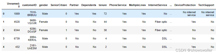
可用pandas的read_csv()函数来读取数据,用DataFrame的head()、shape、info()、duplicated()、nunique()等来初步观察数据。
用户信息可分为个人信息、服务订阅信息和帐单信息三类。
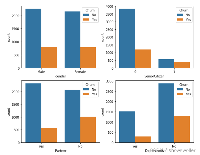
1)个人信息包括gender(性别)、SeniorCitizen(是否老年用户)、Partner(是否伴侣用户)和Dependents(是否亲属用户)。
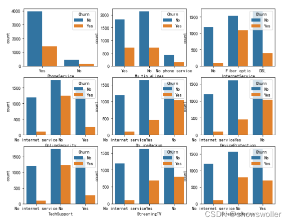
2)服务订阅信息包括tenure(在网时长)、PhoneService(是否开通电话服务业务)、MultipleLines(多线业务服务:Yes,No或No phoneservice)、InternetService(互联网服务:No、DSL数字网络或光纤网络)、OnlineSecurity(网络安全服务:Yes、No或No internetserive)、OnlineBackup(在线备份业务服务:Yes、No或No internetserive)、DeviceProtection(设备保护业务服务:Yes、No或No internetserive)、TechSupport(技术支持服务:Yes、No或No internetserive)、StreamingTV(网络电视服务:Yes、No或No internetserive)、StreamingMovies(网络电影服务:Yes、No或No internetserive)。
3)帐单信息包括Contract(签订合同方式:月、一年或两年)、PaperlessBilling(是否开通电子账单)、PaymentMethod(付款方式:bank transfer、credit card、electronic check或mailed check)、MonthlyCharges(月费用)、TotalCharges(总费用)。
2.流失用户与非流失用户特征分析
1)对于用来描述分类的对象型特征的分布,可用统计图来直观显示。
部分代码如下
import matplotlib.pyplot as plt
import seaborn as sns
fig, axes = plt.subplots(2, 2, figsize=(10, 8))
sns.countplot(x='gender', data=df, hue='Churn', ax=axes[0][0])
sns.countplot(x='SeniorCitizen', data=df, hue='Churn', ax=axes[0][1])
sns.countplot(x='Partner', data=df, hue='Churn', ax=axes[1][0])
sns.countplot(x='Dependents', data=df, hue='Churn', ax=axes[1][1])
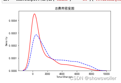
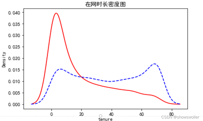
2)对于数值型特征的分布,可用密度图来直观显示
实线表示流失用户,虚线表示非流失用户,可见新用户流失率要高一些
3:分类预测
数据的类型分为对象型和数值型两类。对象型是离散的类别数据,需要对它们进行编码才能形成训练模型的特征。
如果是二值的对象型数据,可以直接用0和1来对它们进行编码。如果取值类别个数多于2,一般可用独热编码。
对于需要进行距离计算的模型,一般还需要对数值型特征进行归一化处理或标准化处理。
经过上述处理后,采用保持法将训练样本切分为训练集和验证集,用来建模并验证模型。
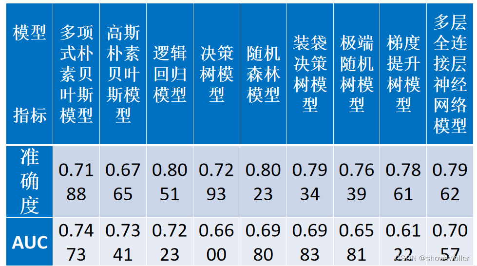
各种方法的准确度及AUC如下
部分代码如下
#!/usr/bin/env python
# coding: utf-8

# ## 1.加载数据,初步观察

# In[1]:


import pandas as pd
import numpy as np


# 观察各特征的类型,是否有缺失值
df.info()


# 各特征含义为:customerID:用户ID;
# gender:性别(Female & Male);
# SeniorCitizen:老年用户(1表示是,0表示不是);
# Partner:伴侣用户(Yes or No);
# Dependents:亲属用户(Yes or No);
# tenure:在网时长(0-72月);
# PhoneService:是否开通电话服务业务(Yes or No);
# MultipleLines:是否开通了多线业务(Yes 、No or No phoneservice 三种);
# InternetService:是否开通互联网服务 (No, DSL数字网络,fiber optic光纤网络 三种);
# OnlineSecurity:是否开通网络安全服务(Yes,No,No internetserive 三种);
# OnlineBackup:是否开通在线备份业务(Yes,No,No internetserive 三种);
# DeviceProtection:是否开通了设备保护业务(Yes,No,No internetserive 三种);
# TechSupport:是否开通了技术支持服务(Yes,No,No internetserive 三种);
# StreamingTV:是否开通网络电视(Yes,No,No internetserive 三种);
# StreamingMovies:是否开通网络电影(Yes,No,No internetserive 三种);
# Contract:签订合同方式 (按月,一年,两年);
# PaperlessBilling:是否开通电子账单(Yes or No);
# PaymentMethod:付款方式(bank transfer,credit card,electronic check,mailed check);
# MonthlyCharges:月费用;
# TotalCharges:总费用;
# Churn:该用户是否流失(Yes or No)。

# In[6]:


# 观察是否有重复值
df.customerID.duplicated().sum()


# In[7]:


# 观察特征的取值情况
df.nunique()


# In[8]:


# 观察下各对象型特征的取值
print('gender : ', set(df['gender']))
print('Partner : ', set(df['Partner']))
print('Dependents : ', set(df['Dependents']))
print('PhoneService : ', set(df['PhoneService']))
print('MultipleLines : ', set(df['MultipleLines']))
print('InternetService : ', set(df['InternetService']))
print('OnlineSecurity : ', set(df['OnlineSecurity']))
print('OnlineBackup : ', set(df['OnlineBackup']))
print('DeviceProtection : ', set(df['DeviceProtection']))
print('TechSupport : ', set(df['TechSupport']))
print('StreamingTV : ', set(df['StreamingTV']))
print('StreamingMovies : ', set(df['StreamingMovies']))
print('Contract : ', set(df['Contract']))
print('PaperlessBilling : ', set(df['PaperlessBilling']))
print('PaymentMethod : ', set(df['PaymentMethod']))
print('Churn : ', set(df['Churn']))


# ## 2.流失用户与非流失用户特征分析

# ### 2.1流失用户与非流失用户的个人信息对比

# In[9]:


import matplotlib.pyplot as plt
import seaborn as sns
fig, axes = plt.subplots(2, 2, figsize=(10, 8))
sns.countplot(x='gender', data=df, hue='Churn', ax=axes[0][0])
sns.countplot(x='SeniorCitizen', data=df, hue='Churn', ax=axes[0][1])
sns.countplot(x='Partner', data=df, hue='Churn', ax=axes[1][0])
sns.countplot(x='Dependents', data=df, hue='Churn', ax=axes[1][1])


# ### 2.2流失用户与非流失用户的服务订阅信息对比

# In[10]:


plt.rc('font', family='SimHei')
plt.title("在网时长密度图")
ax1 = sns.kdeplot(df[df['Churn'] == 'Yes']['tenure'], color='r', linestyle='-', label='Churn:Yes')
ax1 = sns.kdeplot(df[df['Churn'] == 'No']['tenure'], color='b', linestyle='--', label='Churn:No')


# In[11]:


fig, axes = plt.subplots(3, 3, figsize=(10, 8))
sns.countplot(x='PhoneService', data=df, hue='Churn', ax=axes[0][0])
sns.countplot(x='MultipleLines', data=df, hue='Churn', ax=axes[0][1])
sns.countplot(x='InternetService', data=df, hue='Churn', ax=axes[0][2])
sns.countplot(x='OnlineSecurity', data=df, hue='Churn', ax=axes[1][0])
sns.countplot(x='OnlineBackup', data=df, hue='Churn', ax=axes[1][1])
sns.countplot(x='DeviceProtection', data=df, hue='Churn', ax=axes[1][2])
sns.countplot(x='TechSupport', data=df, hue='Churn', ax=axes[2][0])
sns.countplot(x='StreamingTV', data=df, hue='Churn', ax=axes[2][1])
sns.countplot(x='StreamingMovies', data=df, hue='Churn', ax=axes[2][2])


# ### 2.3流失用户与非流失用户帐单信息对比

# In[12]:


fig, axes = plt.subplots(1, 2, figsize=(10, 4))
sns.countplot(x='Contract', data=df, hue='Churn', ax=axes[0])
sns.countplot(x='PaperlessBilling', data=df, hue='Churn', ax=axes[1])


# In[13]:


sns.countplot(x='PaymentMethod', data=df, hue='Churn')


# In[14]:


plt.title("月费用密度图")
ax1 = sns.kdeplot(df[df['Churn'] == 'Yes']['MonthlyCharges'], color='r', linestyle='-', label='Churn:Yes')
ax1 = sns.kdeplot(df[df['Churn'] == 'No']['MonthlyCharges'], color='b', linestyle='--', label='Churn:No')


# In[15]:


# 尝试转化为数值
df.TotalCharges = pd.to_numeric(df.TotalCharges, errors="raise")


# In[16]:


# 根据报错提示,观察下空格字符串的分布
df[df.TotalCharges == " "]


# In[17]:


# 用0代替空字符串,重新尝试
df['TotalCharges'] = df['TotalCharges'].replace(" ", 0)
df.TotalCharges = pd.to_numeric(df.TotalCharges, errors="raise")


# In[18]:


plt.title("总费用密度图")
ax1 = sns.kdeplot(df[df['Churn'] == 'Yes']['TotalCharges'], color='r', linestyle='-', label='Churn:Yes')
ax1 = sns.kdeplot(df[df['Churn'] == 'No']['TotalCharges'], color='b', linestyle='--', label='Churn:No')


# ## 3.分类预测

# ### 3.1 编码,提取特征

# In[19]:


df_clu = df.drop(['Unnamed: 0', 'customerID', 'Churn'], axis=1)
labels = df['Churn']


# In[20]:


# 二值对象型特征转换成数值型
df_clu['gender'] = df_clu['gender'].replace('Male', 1).replace('Female', 0)
df_clu['Partner'] = df_clu['Partner'].replace('Yes', 1).replace('No', 0)
df_clu['Dependents'] = df_clu['Dependents'].replace('Yes', 1).replace('No', 0)
df_clu['PhoneService'] = df_clu['PhoneService'].replace('Yes', 1).replace('No', 0)
df_clu['PaperlessBilling'] = df_clu['PaperlessBilling'].replace('Yes', 1).replace('No', 0)
labels = labels.replace('Yes', 1).replace('No', 0)


# In[21]:


# 离散的,可用距离度量的对象型特征转化为数值型
df_clu['Contract'] = df_clu['Contract'].replace("Month-to-month", 1).replace("One year", 12).replace("Two year", 24)


# In[22]:


# 离散的,不宜用距离度量的特征用one-hot编码
df_clu = pd.get_dummies(df_clu)
df_clu.info()


# In[23]:


df_clu.max()


# In[24]:


# 数据归一化
df_clu['tenure'] = ( df_clu['tenure'] - df_clu['tenure'].min() )/( df_clu['tenure'].max() - df_clu['tenure'].min() )
df_clu['Contract'] = ( df_clu['Contract'] - df_clu['Contract'].min() )/( df_clu['Contract'].max() - df_clu['Contract'].min() )
df_clu['MonthlyCharges'] = ( df_clu['MonthlyCharges'] - df_clu['MonthlyCharges'].min() )/( df_clu['MonthlyCharges'].max() - df_clu['MonthlyCharges'].min() )
df_clu['TotalCharges'] = ( df_clu['TotalCharges'] - df_clu['TotalCharges'].min() )/( df_clu['TotalCharges'].max() - df_clu['TotalCharges'].min() )


# ### 3.2 保持法切分训练集和验证集

# In[25]:


from sklearn.model_selection import train_test_split
from sklearn.metrics import accuracy_score, classification_report, roc_auc_score

# 将数据集分成训练集和验证集
X_train, X_test, y_train, y_test = train_test_split(df_clu, labels, test_size=0.3, random_state = 1026)


# ### 3.3 建模并验证

# In[26]:


# 多项式朴素贝叶斯模型
from sklearn.naive_bayes import MultinomialNB
model = MultinomialNB()
model.fit(X_train, y_train)

predictions = model.predict(X_test)
print('Test set accuracy score: ', accuracy_score(y_test, predictions))
print('Area under the ROC curve: ', roc_auc_score(y_test, predictions))
print(classification_report(y_test, predictions))


# In[27]:


# 高期朴素贝叶斯模型
from sklearn.naive_bayes import GaussianNB
model = GaussianNB()
model.fit(X_train, y_train)

predictions = model.predict(X_test)
print('Test set accuracy score: ', accuracy_score(y_test, predictions))
print('Area under the ROC curve: ', roc_auc_score(y_test, predictions))
print(classification_report(y_test, predictions))


# In[28]:


# 逻辑回归模型
from sklearn.linear_model import LogisticRegression
model = LogisticRegression(solver='liblinear', penalty='l1')
'''
solver:一个字符串,指定了求解最优化问题的算法,可以为如下的值:
'newton-cg':使用牛顿法。
'lbfgs':使用L-BFGS拟牛顿法。
'liblinear' :使用 liblinear。
'sag':使用 Stochastic Average Gradient descent 算法。
'''
model.fit(X_train, y_train)

predictions = model.predict(X_test)
print('Test set accuracy score: ', accuracy_score(y_test, predictions))
print('Area under the ROC curve: ', roc_auc_score(y_test, predictions))
print(classification_report(y_test, predictions))


# In[29]:


# 决策树模型
from sklearn.tree import DecisionTreeClassifier
model = DecisionTreeClassifier(random_state=1026)
model.fit(X_train, y_train)

predictions = model.predict(X_test)
print('Test set accuracy score: ', accuracy_score(y_test, predictions))
print('Area under the ROC curve: ', roc_auc_score(y_test, predictions))
print(classification_report(y_test, predictions))


# In[30]:


# 决策树模型给出的特征重要性
model.feature_importances_


# In[31]:


# 随机森林模型
from sklearn.ensemble import RandomForestClassifier
model = RandomForestClassifier(n_estimators=10, random_state=1026)
model.fit(X_train, y_train)

predictions = model.predict(X_test)
print('Test set accuracy score: ', accuracy_score(y_test, predictions))
print('Area under the ROC curve: ', roc_auc_score(y_test, predictions))
print(classification_report(y_test, predictions))


# In[32]:


# 随机森林模型给出的特征重要性
model.feature_importances_


# In[33]:


# 装袋决策树模型
from sklearn.ensemble import BaggingClassifier
model = BaggingClassifier(n_estimators=10, random_state=1026)
model.fit(X_train, y_train)

predictions = model.predict(X_test)
print('Test set accuracy score: ', accuracy_score(y_test, predictions))
print('Area under the ROC curve: ', roc_auc_score(y_test, predictions))
print(classification_report(y_test, predictions))


# In[34]:


# 极端随机树模型
from sklearn.ensemble import ExtraTreesClassifier
model = ExtraTreesClassifier(n_estimators=10, random_state=1026)
model.fit(X_train, y_train)

predictions = model.predict(X_test)
print('Test set accuracy score: ', accuracy_score(y_test, predictions))
print('Area under the ROC curve: ', roc_auc_score(y_test, predictions))
print(classification_report(y_test, predictions))


# In[35]:


# 梯度提升树模型
from sklearn.ensemble import GradientBoostingClassifier
model = GradientBoostingClassifier(n_estimators=10, random_state=1026)
model.fit(X_train, y_train)

predictions = model.predict(X_test)
print('Test set accuracy score: ', accuracy_score(y_test, predictions))
print('Area under the ROC curve: ', roc_auc_score(y_test, predictions))
print(classification_report(y_test, predictions))


# In[162]:


# 多层全连接层神经网络模型-TensorFlow2框架下实现
import tensorflow as tf

tf_model = tf.keras.Sequential([
    tf.keras.layers.Dense(100, activation='relu', input_shape=(38,), kernel_initializer='random_uniform'),
    tf.keras.layers.Dense(100, activation='relu', kernel_initializer='random_uniform'),
    tf.keras.layers.Dense(1, activation='sigmoid', kernel_initializer='random_uniform')
])


# In[163]:


batch_size = 100 # 每批训练样本数(批梯度下降法)
tf_epoch = 10
tf_model.compile(optimizer='adam', loss='mse', metrics=['accuracy'])
tf_model.summary()
tf_model.fit(np.array(X_train), np.array(y_train), validation_data=(np.array(X_test), np.array(y_test)), batch_size=batch_size, epochs=tf_epoch, verbose=1)


# In[164]:


predictions = tf_model.predict(X_test)
predictions = list(np.round(predictions).reshape(-1,1)) # 四舍五入得到预测值

print('Test set accuracy score: ', accuracy_score(y_test, predictions))
print('Area under the ROC curve: ', roc_auc_score(y_test, predictions))
print(classification_report(y_test, predictions))


# In[173]:


# 多层全连接层神经网络模型-MindSpore框架下实现
import mindspore as ms
cl
    def construct(self, x):
        x = self.relu(self.fc1(x))
        x = self.relu(self.fc2(x))
        x = self.sigmoid(self.fc3(x))
        return x

net = ms_mode() # 实例化
net_loss = ms.nn.loss.MSELoss() # 定义损失函数
opt = ms.nn.Adam(params=net.trainable_params(), learning_rate=0.00005) # 定义优化方法
ms_model = ms.Model(net, net_loss, opt) # 将网络结构、损失函数和优化方法进行关联


# In[167]:

yy.append([0, 1])
    else:
        yy.append([1, 0])

yy = np.array(yy).astype(np.float32)


# In[176]:


class DatasetGenerator:
    def __init__(self, X, y):
        self.data = X
        self.label = y

    def __getitem__(self, index):
        return self.data[index], self.label[index]

    def __len__(self):
        return len(self.data)

batch_size = 100 # 每批训练样本数
rain.batch(batch_size)
ds_train = ds_train.repeat(repeat_size)

from mindspore.train.callback import LossMonitor, TimeMonitor
loss_cb = LossMonitor(per_print_times=1)
time_cb = TimeMonitor(data_size=ds_train.get_dataset_size())

ms_epoch = 30
ms_model.train(ms_epoch, ds_train, dataset_sink_mode=False, callbacks=[loss_cb, time_cb])


# In[177]:


# 预测
predictions = []
#xx = X_test.values
for i in range(len(X_test)):
    y_p = ms_model.predict(ms.Tensor([X_test[i]], ms.float32))
    predictions.append(y_p.asnumpy()[0][0]) # 直接取独热编码的第一个值

predictions =  roc_auc_score(y_test, predictions))
print(classification_report(y_test, predictions))


# In[ ]:
创作不易 觉得有帮助请点赞关注收藏~~~


 2万+
2万+


 被折叠的 条评论
为什么被折叠?
被折叠的 条评论
为什么被折叠?
 到【灌水乐园】发言


