DataWhale集成学习-Task6

记录DataWhale集成学习的组队学习过程，Task6算是一个阶段性的总结，用SVM和PCA对LFW这个人脸识别数据集进行分类。这是一个多分类问题，先用PCA降维，再用SVM做分类。sklearn官方有LFW人脸识别的教程，感兴趣的朋友可以在官方文档上仔细的看整个流程。具体代码如下：

import matplotlib.pyplot as plt
from sklearn.model_selection import train_test_split
from sklearn.model_selection import GridSearchCV
from sklearn.datasets import fetch_lfw_people
from sklearn.metrics import classification_report
from sklearn.metrics import confusion_matrix
from sklearn.decomposition import PCA
from sklearn.svm import SVC

# #############################################################################
# 下载数据，选择照片数大于70的做数据集。
# 1288个样本，每个样本特征维度为1850维，多分类问题，共7类。

lfw_people = fetch_lfw_people(min_faces_per_person=70, resize=0.4)
n_samples, h, w = lfw_people.images.shape

# 这里直接把图片flatten成了1850维的特征向量，没考虑像素间的相关性。
X = lfw_people.data
n_features = X.shape[1]

y = lfw_people.target #标签y的代表人类别的整数id。
target_names = lfw_people.target_names #target_names是id代表的具体的名字。
n_classes = target_names.shape[0]


# #############################################################################
# 划分训练集和测试集
X_train, X_test, y_train, y_test = train_test_split(X, y, test_size=0.25, random_state=42)

# #############################################################################
# 原始特征维度太大，使用PCA降维
n_components = 150 #选择前150个主成成分。
pca = PCA(n_components=n_components, svd_solver='randomized',whiten=True).fit(X_train)
eigenfaces = pca.components_.reshape((n_components, h, w))#PCA降维后再reshape成特征脸。

#PCA降维后的特征。
X_train_pca = pca.transform(X_train)
X_test_pca = pca.transform(X_test)

##############################################################################
# 在训练集上使用SVM模型以及网格搜索确定超参数。
# 由于PCA降维后的特征已经是归一化了，所以在SVM上不用再对特征归一化。

param_grid = {'C': [1.29,1.3,1.31,1.32,1.33,1.34],
              'gamma': [0.0043,0.0044,0.0045,0.0046]}
svc= SVC(kernel='rbf', class_weight='balanced') #使用高斯核
clf = GridSearchCV(svc, param_grid,cv=10)
clf = clf.fit(X_train_pca, y_train)

print("网格搜索到的最佳参数:")
print(clf.best_estimator_)


# #############################################################################
# 在测试集上评估模型

y_pred = clf.predict(X_test_pca)

#使用classification_report显示主要分类指标的文本报告
print(classification_report(y_test, y_pred, target_names=target_names))

#混淆矩阵画图
confmat = confusion_matrix(y_test, y_pred) #confmat为7*7的矩阵
fig,ax = plt.subplots()
ax.matshow(confmat, cmap=plt.cm.Blues,alpha=0.8)
for i in range(confmat.shape[0]):
    for j in range(confmat.shape[1]):
        ax.text(x=j,y=i,s=confmat[i,j],va='center',ha='center')
plt.xlabel('predict label')
plt.ylabel('true label')
plt.show()


输出：
                  precision    recall  f1-score   support

     Ariel Sharon       0.64      0.69      0.67        13
     Colin Powell       0.77      0.90      0.83        60
  Donald Rumsfeld       0.86      0.70      0.78        27
    George W Bush       0.91      0.94      0.93       146
Gerhard Schroeder       0.88      0.84      0.86        25
      Hugo Chavez       0.90      0.60      0.72        15
       Tony Blair       0.94      0.83      0.88        36

         accuracy                           0.87       322
        macro avg       0.84      0.79      0.81       322
     weighted avg       0.87      0.87      0.87       322

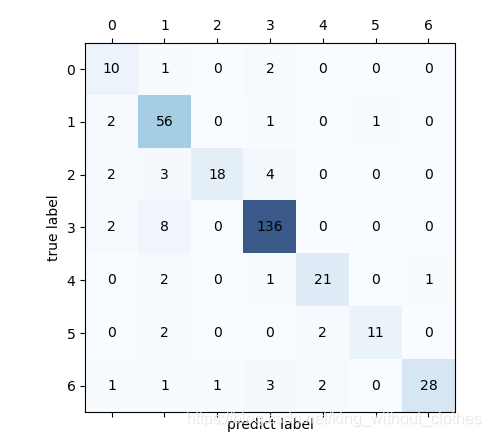
可以看出，简单的PCA+SVM效果还可以，但是我们现在的做法是直接将像素拉伸成了一个高维向量，忽略了像素间的位置信息，使用CNN这种考虑像素间位置信息的模型肯定会取得更好的结果。