


本文整理NMF相关知识。
简介
非负矩阵分解(Nonnegative Matrix Factorization),简称NMF,是由Lee和Seung于1999年在自然杂志上提出的一种矩阵分解方法,它使分解后的所有分量均为非负值(要求纯加性的描述),并且同时实现非线性的维数约减。NMF已逐渐成为信号处理、生物医学工程、模式识别、计算机视觉和图像工程等研究领域中最受欢迎的多维数据处理工具之一。
如果X是一个nxp非负矩阵,NMF就是找到两个矩阵W和H,使得
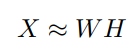
W、H是n×r和r×p的非负矩阵。在实践中,因式分解的rank(级别)通常被选择为r<<min(n, p),其目的是为了将X中包含的信息分成r个因子,也就是W的列。不同领域中矩阵W的名称不同,比如基础图像,元基因,源信号等,而矩阵H可能会称为混合系数矩阵和元基因表达系数等。
算法
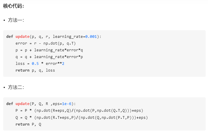
可以通过普通的梯度下降法(SGD),或根据Lee和Seung文章提出的multiplicative update的规则进行计算获取矩阵W和H。
参见: https://zhuanlan.zhihu.com/p/116846017
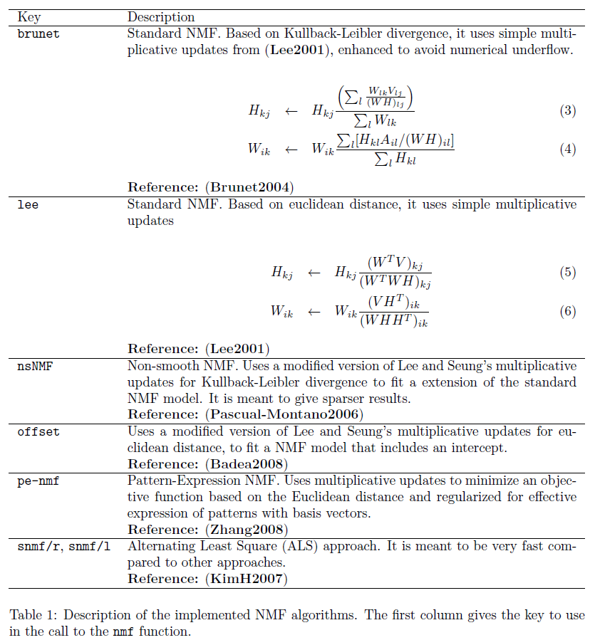
除此之外,R的NMF包内置的算法就有11种之多,(综述Berry2007; Chu2004)。其中默认是brunet,可使用nmfAlgorithm()设定算法。
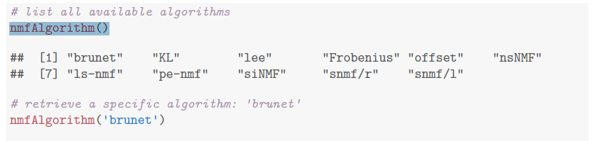
大部分算法由C++执行,也可以选用R执行的版本。
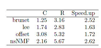
并且可以将算法做成list,对比各种算法的表现。
nmf.res.multi.method <- nmf(nmf.input, rank2use,list('brunet', 'lee', 'ns'), seed=seed2use)
compare(nmf.res.multi.method)
除了内置的算法,NMF包还允许接入其他NMF算法,例如projective NMF(PNMF)
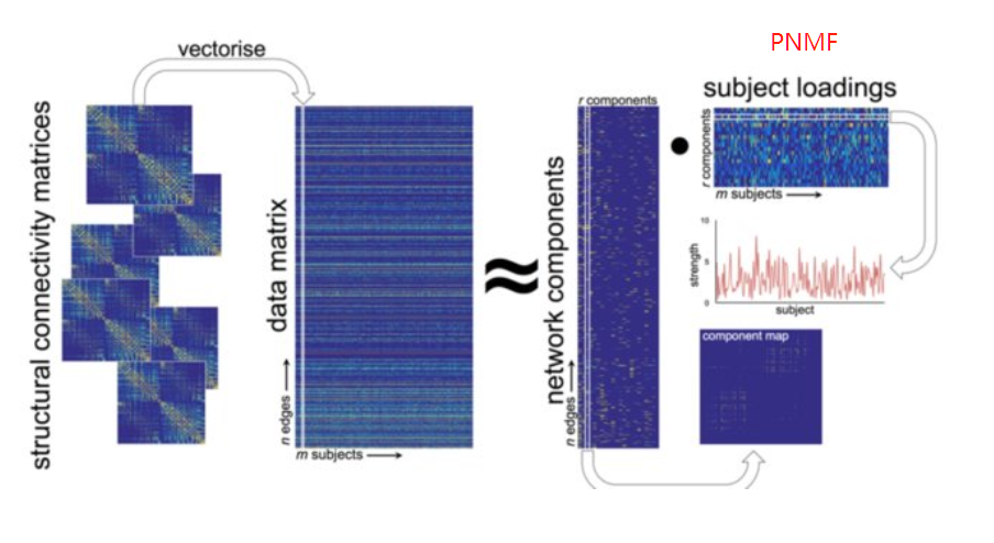
remotes::install_github("richardbeare/pNMF")
library(NMF)
setNMFMethod("PNMF", pNMF::PNMF)
与NMF相比,PNMF算法将H进一步分解,生成一个更稀疏的矩阵,有利于特征提取和聚类(Ball et al HBM2017)。
模型表现
问题一:如何选择rank数目?
相关指标的解释,来自于NMF相关函数说明。

👉Cophenetic correlation
The cophenetic correlation coeffificient is based on the consensus matrix (i.e. the average of connectivity matrices) and was proposed by Brunet et al. (2004) to measure the stability of the clusters obtained from NMF. It is defined as the Pearson correlation between the samples' distances induced by the consensus matrix (seen as a similarity matrix) and their cophenetic distances from a hierachical clustering based on these very distances (by default an average linkage is used). See Brunet et al. (2004).
👉Dispersion coefficent
The dispersion coefficient is based on the consensus matrix (i.e. the average of connectivity matrices) and was proposed by Kim et al. (2007) to measure the reproducibility of the clusters obtained from NMF.
👉evar/residual/rss
Explained variance/residual/residual sum of sqaures
In the context of NMF, Hutchins et al. (2008) used the variation of the RSS in combination with the algorithm from Lee et al. (1999) to estimate the correct number of basis vectors. The optimal rank is chosen where the graph of the RSS first shows an inflexion point, i.e. using a screeplot-type criterium.
Note that this way of estimation may not be suitable for all models. Indeed, if the NMF optimisation problem is not based on the Frobenius norm, the RSS is not directly linked to the quality of approximation of the NMF model. However, it is often the case that it still decreases with the rank.
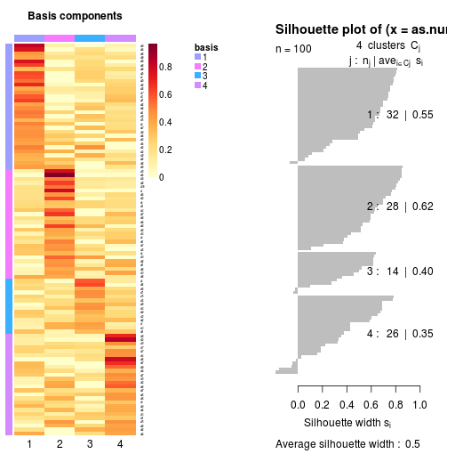
👉Silhouette
Silhouette refers to a method of interpretation and validation of consistency within clusters of data. The technique provides a succinct graphical representation of how well each object has been classified. It was proposed by Belgian statistician Peter Rousseeuw in 1987.
The silhouette value is a measure of how similar an object is to its own cluster (cohesion) compared to other clusters (separation). The silhouette ranges from −1 to +1, where a high value indicates that the object is well matched to its own cluster and poorly matched to neighboring clusters. If most objects have a high value, then the clustering configuration is appropriate. If many points have a low or negative value, then the clustering configuration may have too many or too few clusters.
The silhouette can be calculated with any distance metric, such as the Euclidean distance or the Manhattan distance.
👉Sparseness
The sparseness quantifies how much energy of a vector is packed into only few components (Hoyer; 2004). The sparseness is a real number in [0,1]. It is equal to 1 if and only if X contains a single nonzero component, and is equal to 0 if and only if all components of X are equal. It interpolates smoothly between these two extreme values. The closer to 1 is the sparseness the sparser is the vector.
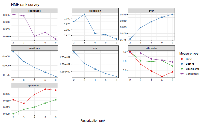
关于选择rank数目的建议,例如,Brunet(2004)建议选择cophenetic开始下降的第一个r值,Hutchins(2008)建议选择RSS曲线出现切点的第一个值。Frigyesi(2008)认为RSS的下降幅度低于从随机数据得到的RSS的下降幅度的最小值,NMF自带了randomize函数可以对每一列进行重采样。另外也可以结合多个指标选择rank数量,例如下图是2021年看到的poster,选择了r=8,此时error小stability高。为什么不选r=10,12,28?需要考虑可解释性和过拟合的问题。
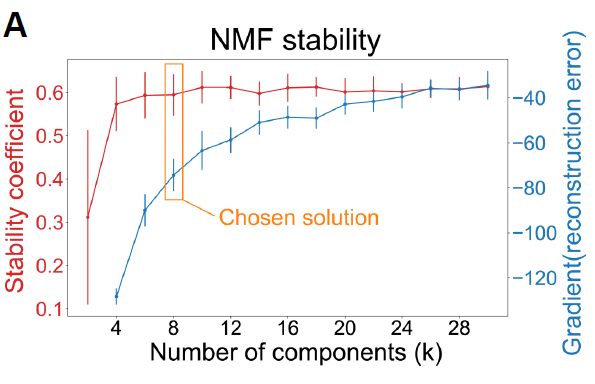
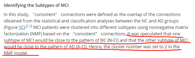
也看到过根据假设或者说故事合不合理来决定,比如做MCI发现一个亚类型更像HC,一个亚类型更像AD,碎石图都不需要了,直接决定r=2
【传送门】
问题二:应该使用多少个run?
一个run代表做一次NMF分解,每一次得到的结果都可能有出入,因此需要多个run。文献(Brunet2004; Hutchins2008)推荐run的数量是30-50,NMF文档另外一个地方推荐的是100-200。结果fit变量中默认保存的是表现最好的一个run的H和W矩阵,如果需要保存所有run的结果,需要设定
.options=list(keep.all=TRUE)作图
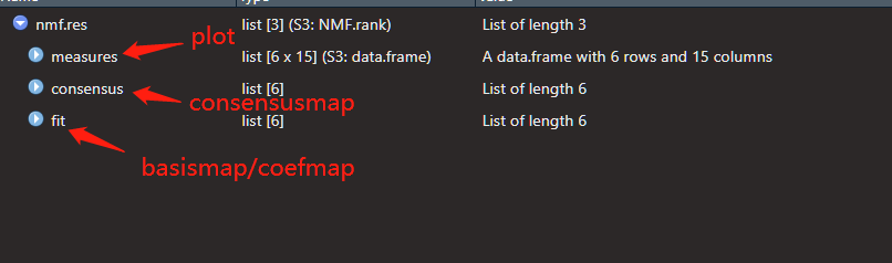
nmf.res为运行结果。
plot(nmf.res)获取的是模型表现的各个指标
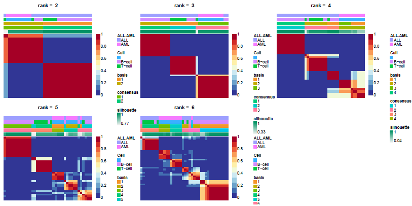
consensusmap(nmf.res)获取多个run之间的一致性。
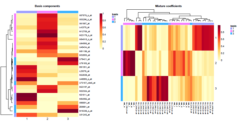
basismap(nmf.res$fit$`3`, subsetRow=TRUE)
coefmap(nmf.res$fit$`3`)
可以绘制相应rank中矩阵W和H的热图
NMF和PCA的区别

都为矩阵分解的方法,约束条件不同,PCA要求分解后矩阵正交,NMF要求分解后矩阵都为正,NMF如果只要求一个矩阵为正,则是semi-NMF,增加L1正则项,则是spase NMF。其中semi-NMF的用处就是可以允许被分解矩阵X中存在负数,对应NMF包设置为mixed=TRUE,有此设置,可以跳过对输入数据的符号检查,使用自定义的semi-NMF算法进行因式分解。
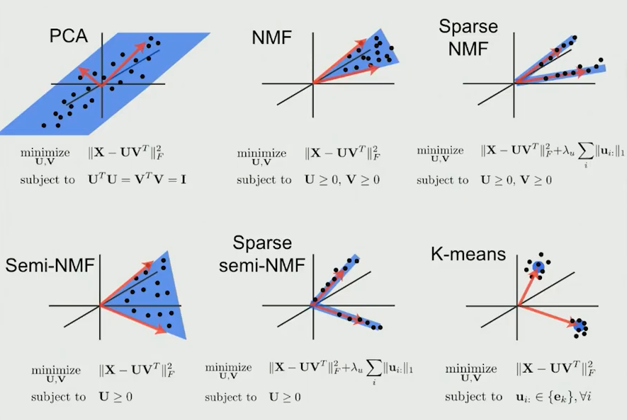
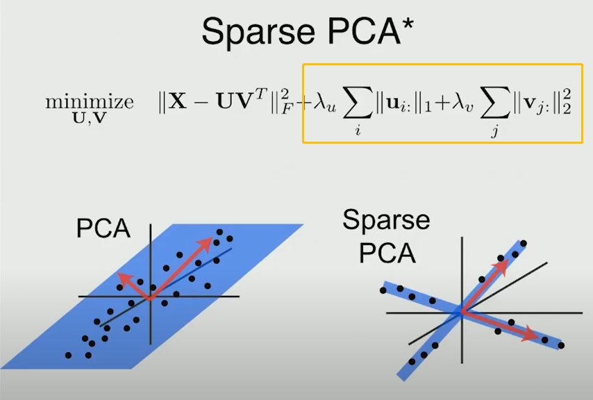
用NMF的一个目的就是得到sparse并且可加的分解结果,便于解释。其实Sparse PCA也有类似的效果,sparse的主轴只和某几个变量相关,提高了在实际使用中的可解释性。
关于NMF在领域内的一些应用,见下一个推送。


 5万+
5万+

 被折叠的 条评论
为什么被折叠?
被折叠的 条评论
为什么被折叠?
 到【灌水乐园】发言


