


目录
4.测试训练好的模型
一、 实现卷积-池化-激活
重新复习一下以前提到的知识:
卷积:在神经网络中,我理解就是像素点和卷积核中的权重相乘再相加,执行卷积的目的是从输入中提取有用的特征。
卷积核:
又称为滤波器,具体就是用来检测某一方面的特征,比如垂直边界、水平边界等特征。
卷积核大小可以指定为小于输入图像尺寸的任意值,卷积核越大,可提取的输入特征越复杂,一般都是三通道。
拿Pytorch官网Conv2d()举例,它的输入输出关系如下:
注:dilated convolution 为空洞卷积,若正常操作使用pooling减小图像尺寸增大感受野,然后upsampling扩大图像尺寸。在先减小再增大尺寸的过程中,肯定有一些信息损失掉了。dilated convolution的作用就是不做pooling损失信息的情况下,加大感受野,让每个卷积输出都包含较大范围的信息。
池化:池化操作是CNN中非常常见的一种操作,Pooling层是模仿人的视觉系统对数据进行降维,池化操作通常也叫做子采样或降采样,在构建卷积神经网络时,往往会用在卷积层之后,通过池化来降低卷积层输出的特征维度,有效减少网络参数的同时还可以防止过拟合现象。
主要功能就是:
- 抑制噪声,降低信息冗余
- 提升模型的尺度不变性、旋转不变形
- 降低模型计算量
- 防止过拟合
下面是最大池化官网定义: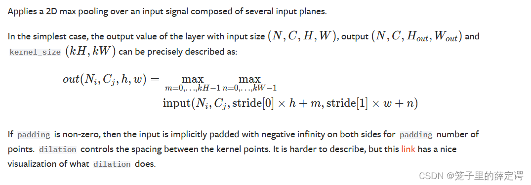
下面是池化层的一些参数和输出尺寸(空洞参数在上文已经解释):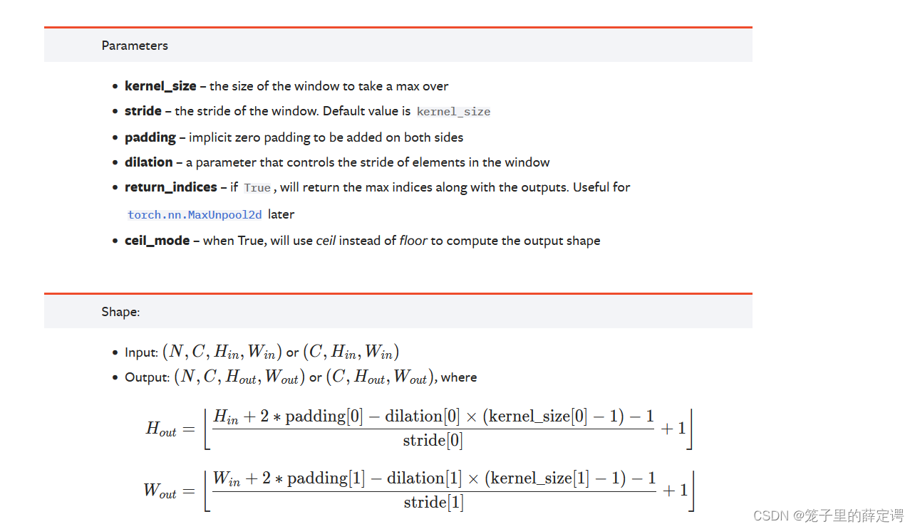
扩展:一提到池化操作,大部分人第一想到的就是maxpool和avgpool,实际上还有很多种池化操作。
(1). 最大/平均池化
最大池化就是选择图像区域中最大值作为该区域池化以后的值,反向传播的时候,梯度通过前向传播过程的最大值反向传播,其他位置梯度为0。
使用的时候,最大池化又分为重叠池化和非重叠池化,比如常见的stride=kernel size的情况属于非重叠池化,如果stride<kernel size 则属于重叠池化。重叠池化相比于非重叠池化不仅可以提升预测精度,同时在一定程度上可以缓解过拟合。
重叠池化一个应用的例子就是yolov3-tiny的backbone最后一层,使用了一个stride=1, kernel size=2的maxpool进行特征的提取。
平均池化就是将选择的图像区域中的平均值作为该区域池化以后的值。
(2). 随机池化
如下图所示,特征区域的大小越大,代表其被选择的概率越高,比如左下角的本应该是选择7,但是由于引入概率,5也有一定几率被选中。
《Stochastic Pooling for Regularization of Deep Convolutional Neural Networks》这篇论文已经证明了使用随机池化效果和采用dropout的结果接近,证明了其有一定防止过拟合的作用。
(3).组合池化
组合池化则是同时利用最大值池化与均值池化两种的优势而引申的一种池化策略。常见组合策略有两种:Cat与Add。常常被当做分类任务的一个trick,其作用就是丰富特征层,maxpool更关注重要的局部特征,而average pooling更关注全局特征。
(4).Spatial Pyramid Pooling
这是何凯明大神(巨佬)在SPPNet中提出,用于解决重复卷积计算和固定输出的两个问题,即多个空间池化的组合,对不同输出尺度采用不同的划窗大小和步长以确保输出尺度相同,同时能够融合金字塔提取出的多种尺度特征,能够提取更丰富的语义信息。常用于多尺度训练和目标检测中的RPN网络。
上个学期我跑了一下用于物体检测的YOLOV3,其中就有yolov3-spp这一网络结构,通过spp模块实现局部特征和全局特征(所以空间金字塔池化结构的最大的池化核要尽可能的接近等于需要池化的featherMap的大小)的featherMap级别的融合,丰富最终特征图的表达能力,从而提高MAP。但是我没有训练好这一网络结构,在上个学期训练出的最后结果还挺烂的,还有机会公费炼丹的话一定再试试。
从感受野角度来讲,之前计算感受野的时候可以明显发现,maxpool的操作对感受野的影响非常大,其中主要取决于kernel size大小。在SPP中,使用了kernel size非常大的maxpool会极大提高模型的感受野。
其余请自行了解。
激活:这个已经在前馈神经网络解释烂了,在卷积神经网络中的定义和前馈神经网络基本一致,就是将前一层的线性输出,通过非线性的激活函数进行处理,这样用以模拟任意函数,从而增强网络的表征能力,具体解释看前面的博客。
1.Nmupy版本:手工实现 卷积-池化-激活
import numpy as np
import matplotlib.pyplot as plt
plt.rcParams['font.sans-serif'] = ['SimHei'] # 用来正常显示中文标签
plt.rcParams['axes.unicode_minus'] = False # 用来正常显示负号
x = np.array([[-1, -1, -1, -1, -1, -1, -1, -1, -1],
[-1, 1, -1, -1, -1, -1, -1, 1, -1],
[-1, -1, 1, -1, -1, -1, 1, -1, -1],
[-1, -1, -1, 1, -1, 1, -1, -1, -1],
[-1, -1, -1, -1, 1, -1, -1, -1, -1],
[-1, -1, -1, 1, -1, 1, -1, -1, -1],
[-1, -1, 1, -1, -1, -1, 1, -1, -1],
[-1, 1, -1, -1, -1, -1, -1, 1, -1],
[-1, -1, -1, -1, -1, -1, -1, -1, -1]])
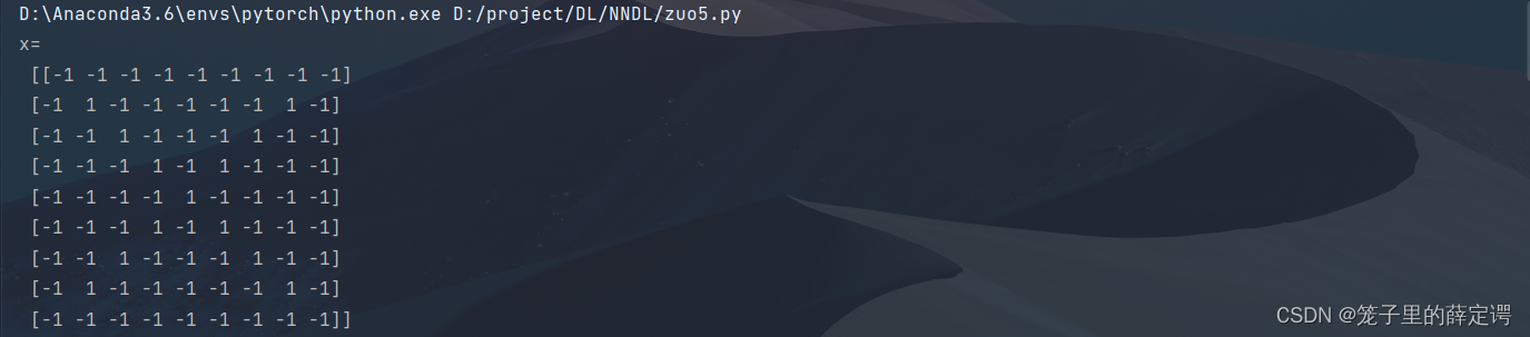
print("x=\n", x)
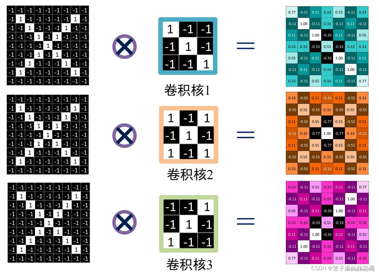
# 初始化 三个 卷积核
Kernel = [[0 for i in range(0, 3)] for j in range(0, 3)]
Kernel[0] = np.array([[1, -1, -1],
[-1, 1, -1],
[-1, -1, 1]])
Kernel[1] = np.array([[1, -1, 1],
[-1, 1, -1],
[1, -1, 1]])
Kernel[2] = np.array([[-1, -1, 1],
[-1, 1, -1],
[1, -1, -1]])
plt.figure(1, figsize=[50, 50], edgecolor='c', facecolor='c')
plt.subplots_adjust(left=None, bottom=None, right=None, top=None, wspace=0.15, hspace=0.5)
plt.subplot(331).set_title('原图')
plt.imshow(x, cmap=plt.cm.hot, vmin=-1, vmax=1)
plt.colorbar()
plt.subplot(332).set_title('卷积核1')
plt.colorbar()
plt.imshow(Kernel[0], cmap=plt.cm.hot, vmin=-1, vmax=1)
plt.subplot(333).set_title('卷积核2')
plt.colorbar()
plt.imshow(Kernel[1], cmap=plt.cm.hot, vmin=-1, vmax=1)
plt.subplot(334).set_title('卷积核3')
plt.colorbar()
plt.imshow(Kernel[2], cmap=plt.cm.hot, vmin=-1, vmax=1)
# --------------- 卷积 ---------------
stride = 1 # 步长
feature_map_h = 7 # 特征图的高
feature_map_w = 7 # 特征图的宽
feature_map = [0 for i in range(0, 3)] # 初始化3个特征图
for i in range(0, 3):
feature_map[i] = np.zeros((feature_map_h, feature_map_w)) # 初始化特征图
for h in range(feature_map_h): # 向下滑动,得到卷积后的固定行
for w in range(feature_map_w): # 向右滑动,得到卷积后的固定行的列
v_start = h * stride # 滑动窗口的起始行(高)
v_end = v_start + 3 # 滑动窗口的结束行(高)
h_start = w * stride # 滑动窗口的起始列(宽)
h_end = h_start + 3 # 滑动窗口的结束列(宽)
window = x[v_start:v_end, h_start:h_end] # 从图切出一个滑动窗口
for i in range(0, 3):
feature_map[i][h, w] = np.divide(np.sum(np.multiply(window, Kernel[i][:, :])), 9)
print("feature_map:\n", np.around(feature_map, decimals=2))
plt.subplot(335).set_title('卷积核1卷积结果')
plt.colorbar()
plt.imshow(feature_map[0], cmap=plt.cm.hot, vmin=-1, vmax=1)
plt.subplot(336).set_title('卷积核2卷积结果')
plt.colorbar()
plt.imshow(feature_map[1], cmap=plt.cm.hot, vmin=-1, vmax=1)
plt.subplot(337).set_title('卷积核3卷积结果')
plt.colorbar()
plt.imshow(feature_map[2], cmap=plt.cm.hot, vmin=-1, vmax=1)
# --------------- 池化 ---------------
pooling_stride = 2 # 步长
pooling_h = 4 # 特征图的高
pooling_w = 4 # 特征图的宽
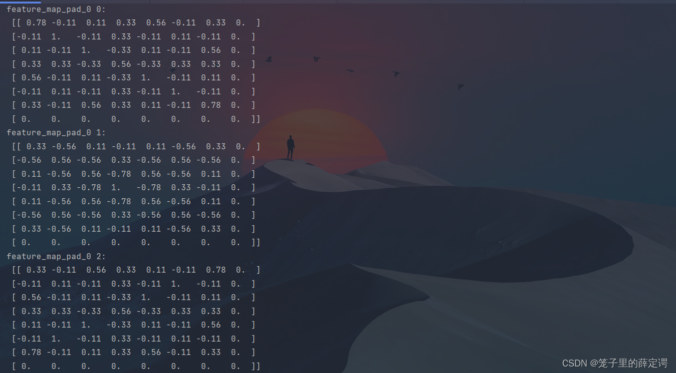
feature_map_pad_0 = [[0 for i in range(0, 8)] for j in range(0, 8)]
for i in range(0, 3): # 特征图 补 0 ,行 列 都要加 1 (因为上一层是奇数,池化窗口用的偶数)
feature_map_pad_0[i] = np.pad(feature_map[i], ((0, 1), (0, 1)), 'constant', constant_values=(0, 0))
print("feature_map_pad_0 0:\n", np.around(feature_map_pad_0[0], decimals=2))
print("feature_map_pad_0 1:\n", np.around(feature_map_pad_0[1], decimals=2))
print("feature_map_pad_0 2:\n", np.around(feature_map_pad_0[2], decimals=2))
plt.figure(2, figsize=[50, 50], edgecolor='c', facecolor='c')
plt.subplot(331).set_title('特征图1补零结果')
plt.imshow(feature_map_pad_0[0], cmap=plt.cm.hot, vmin=-1, vmax=1)
plt.colorbar()
plt.subplot(332).set_title('特征图2补零结果')
plt.colorbar()
plt.imshow(feature_map_pad_0[1], cmap=plt.cm.hot, vmin=-1, vmax=1)
plt.subplot(333).set_title('特征图3补零结果')
plt.colorbar()
plt.imshow(feature_map_pad_0[2], cmap=plt.cm.hot, vmin=-1, vmax=1)
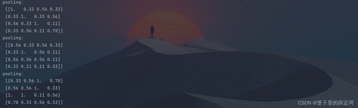
pooling = [0 for i in range(0, 3)]
for i in range(0, 3):
pooling[i] = np.zeros((pooling_h, pooling_w)) # 初始化特征图
for h in range(pooling_h): # 向下滑动,得到卷积后的固定行
for w in range(pooling_w): # 向右滑动,得到卷积后的固定行的列
v_start = h * pooling_stride # 滑动窗口的起始行(高)
v_end = v_start + 2 # 滑动窗口的结束行(高)
h_start = w * pooling_stride # 滑动窗口的起始列(宽)
h_end = h_start + 2 # 滑动窗口的结束列(宽)
for i in range(0, 3):
pooling[i][h, w] = np.max(feature_map_pad_0[i][v_start:v_end, h_start:h_end])
print("pooling:\n", np.around(pooling[0], decimals=2))
print("pooling:\n", np.around(pooling[1], decimals=2))
print("pooling:\n", np.around(pooling[2], decimals=2))
plt.subplot(334).set_title('特征图1补零后池化结果')
plt.colorbar()
plt.imshow(pooling[0], cmap=plt.cm.hot, vmin=-1, vmax=1)
plt.subplot(335).set_title('特征图2补零后池化结果')
plt.colorbar()
plt.imshow(pooling[1], cmap=plt.cm.hot, vmin=-1, vmax=1)
plt.subplot(336).set_title('特征图3补零后池化结果')
plt.colorbar()
plt.imshow(pooling[2], cmap=plt.cm.hot, vmin=-1, vmax=1)
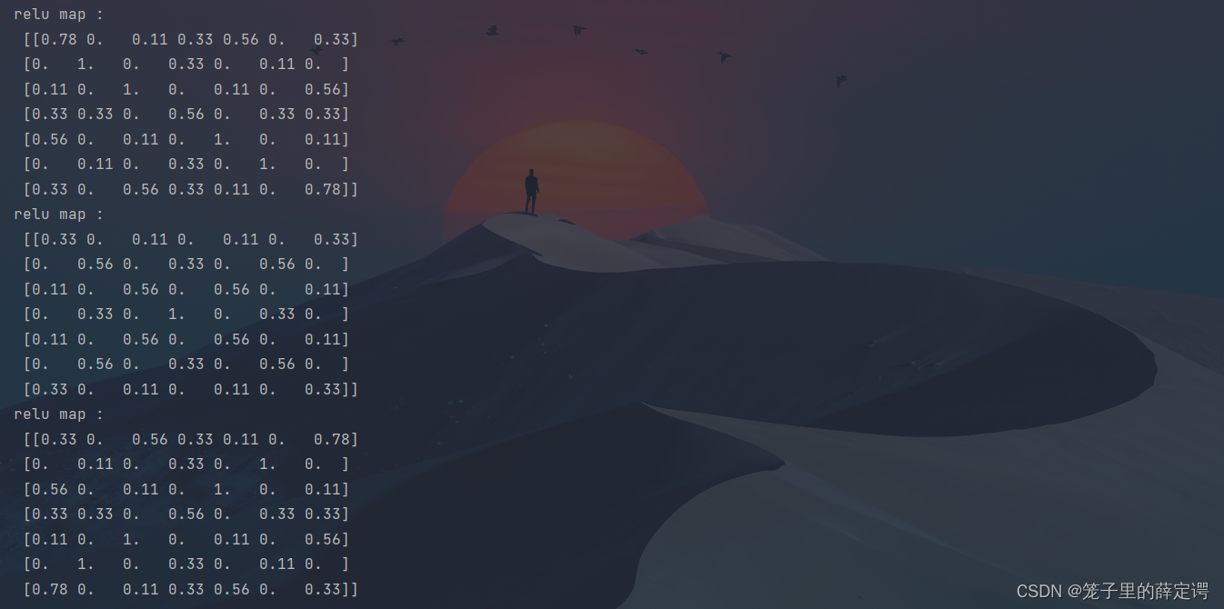
# --------------- 激活 ---------------
def relu(x):
return (abs(x) + x) / 2
relu_map_h = 7 # 特征图的高
relu_map_w = 7 # 特征图的宽
relu_map = [0 for i in range(0, 3)] # 初始化3个特征图
for i in range(0, 3):
relu_map[i] = np.zeros((relu_map_h, relu_map_w)) # 初始化特征图
for i in range(0, 3):
relu_map[i] = relu(feature_map[i])
print("relu map :\n", np.around(relu_map[0], decimals=2))
print("relu map :\n", np.around(relu_map[1], decimals=2))
print("relu map :\n", np.around(relu_map[2], decimals=2))
plt.subplot(337).set_title('池化1后使用Relu激活结果')
plt.colorbar()
plt.imshow(relu_map[0], cmap=plt.cm.hot, vmin=-1, vmax=1)
plt.subplot(338).set_title('池化2后使用Relu激活结果')
plt.colorbar()
plt.imshow(relu_map[1], cmap=plt.cm.hot, vmin=-1, vmax=1)
plt.subplot(339).set_title('池化3后使用Relu激活结果')
plt.imshow(relu_map[2], cmap=plt.cm.hot, vmin=-1, vmax=1)
plt.colorbar()
plt.show()
运行结果:
 可视化:
可视化: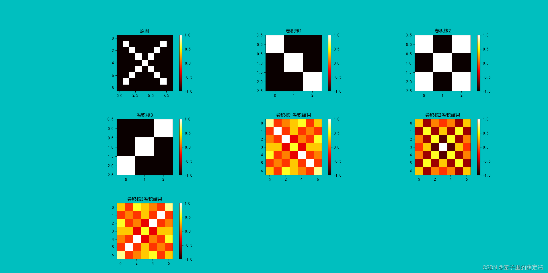
 可视化:
可视化: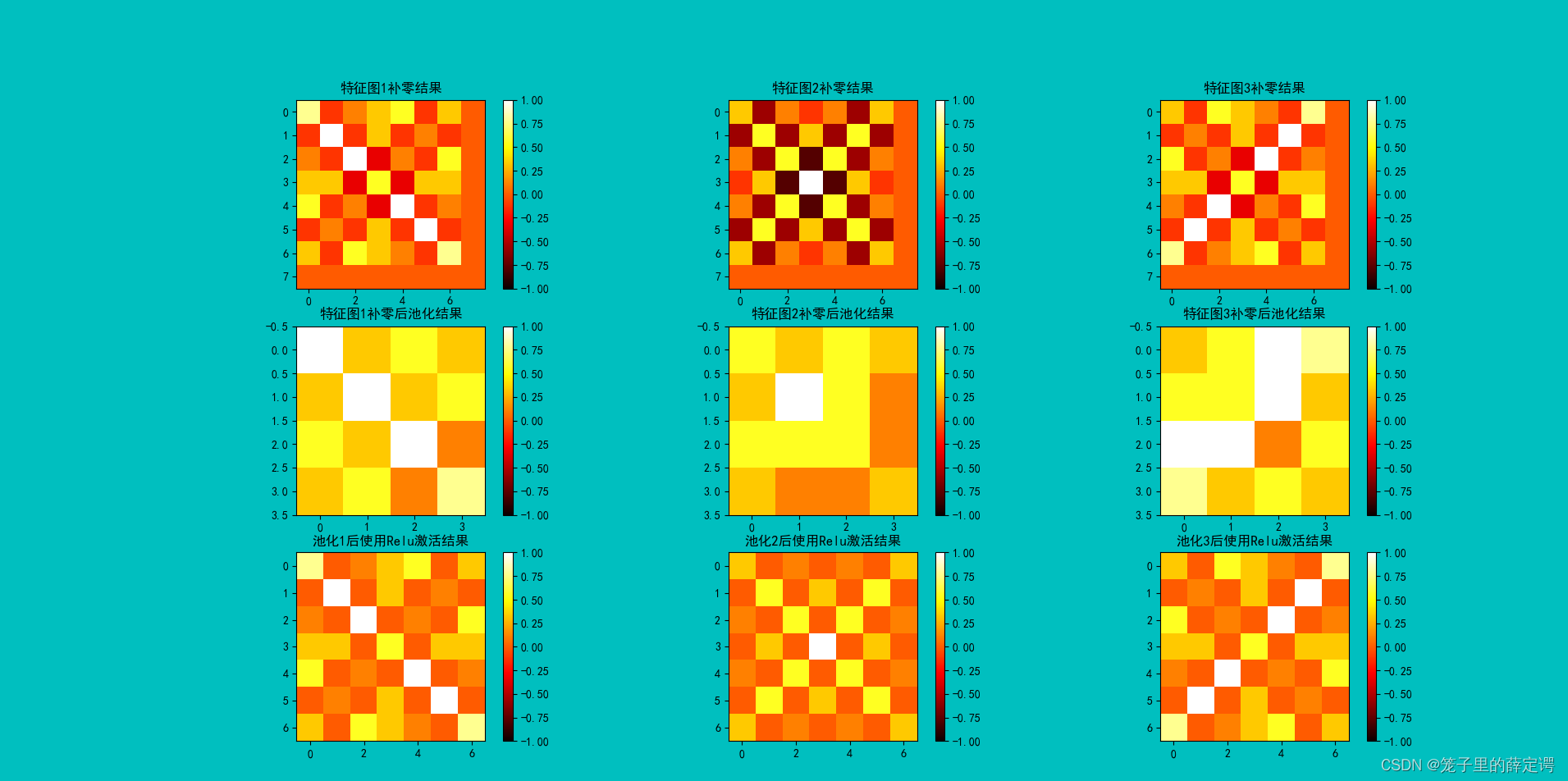
2.Pytorch版本:调用函数实现 卷积-池化-激活
import torch
import torch.nn as nn
import matplotlib.pyplot as plt
plt.rcParams['font.sans-serif'] = ['SimHei'] # 用来正常显示中文标签
plt.rcParams['axes.unicode_minus'] = False # 用来正常显示负号 #有中文出现的情况,需要u'内容
x = torch.tensor([[[[-1, -1, -1, -1, -1, -1, -1, -1, -1],
[-1, 1, -1, -1, -1, -1, -1, 1, -1],
[-1, -1, 1, -1, -1, -1, 1, -1, -1],
[-1, -1, -1, 1, -1, 1, -1, -1, -1],
[-1, -1, -1, -1, 1, -1, -1, -1, -1],
[-1, -1, -1, 1, -1, 1, -1, -1, -1],
[-1, -1, 1, -1, -1, -1, 1, -1, -1],
[-1, 1, -1, -1, -1, -1, -1, 1, -1],
[-1, -1, -1, -1, -1, -1, -1, -1, -1]]]], dtype=torch.float)
print(x.shape)
print(x)
img = x.data.squeeze().numpy() # 将输出转换为图片的格式
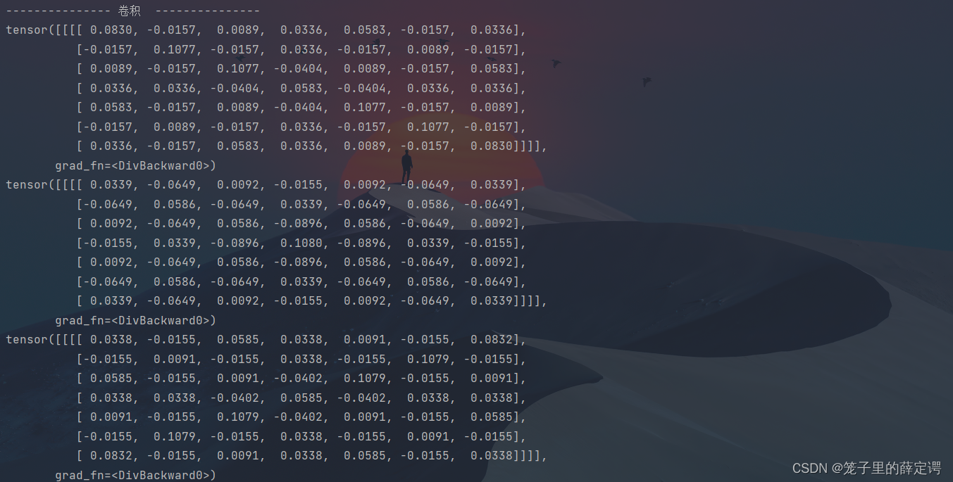
print("--------------- 卷积 ---------------")
conv1 = nn.Conv2d(1, 1, (3, 3), 1) # in_channel , out_channel , kennel_size , stride
conv1.weight.data = torch.Tensor([[[[1, -1, -1],
[-1, 1, -1],
[-1, -1, 1]]
]])
img2 = conv1.weight.data.squeeze().numpy() # 将输出转换为图片的格式
conv2 = nn.Conv2d(1, 1, (3, 3), 1) # in_channel , out_channel , kennel_size , stride
conv2.weight.data = torch.Tensor([[[[1, -1, 1],
[-1, 1, -1],
[1, -1, 1]]
]])
img3 = conv2.weight.data.squeeze().numpy() # 将输出转换为图片的格式
conv3 = nn.Conv2d(1, 1, (3, 3), 1) # in_channel , out_channel , kennel_size , stride
conv3.weight.data = torch.Tensor([[[[-1, -1, 1],
[-1, 1, -1],
[1, -1, -1]]
]])
img4 = conv3.weight.data.squeeze().numpy() # 将输出转换为图片的格式
plt.figure(1, figsize=[50, 50], edgecolor='c', facecolor='c')
plt.subplot(331).set_title('原图')
plt.imshow(img, cmap=plt.cm.hot, vmin=-1, vmax=1)
plt.subplot(332).set_title('卷积核1')
plt.imshow(img2, cmap=plt.cm.hot, vmin=-1, vmax=1)
plt.subplot(333).set_title('卷积核2')
plt.imshow(img3, cmap=plt.cm.hot, vmin=-1, vmax=1)
plt.subplot(334).set_title('卷积核3')
plt.imshow(img4, cmap=plt.cm.hot, vmin=-1, vmax=1)
feature_map1 = conv1(x) / 9
feature_map2 = conv2(x) / 9
feature_map3 = conv3(x) / 9
print(feature_map1 / 9)
print(feature_map2 / 9)
print(feature_map3 / 9)
img5 = feature_map1.data.squeeze().numpy() # 将输出转换为图片的格式
img6 = feature_map1.data.squeeze().numpy() # 将输出转换为图片的格式
img7 = feature_map1.data.squeeze().numpy() # 将输出转换为图片的格式
plt.subplot(335).set_title('卷积核1卷积结果')
plt.imshow(img5, cmap=plt.cm.hot, vmin=-1, vmax=1)
plt.subplot(336).set_title('卷积核2卷积结果')
plt.imshow(img6, cmap=plt.cm.hot, vmin=-1, vmax=1)
plt.subplot(337).set_title('卷积核3卷积结果')
plt.imshow(img7, cmap=plt.cm.hot, vmin=-1, vmax=1)
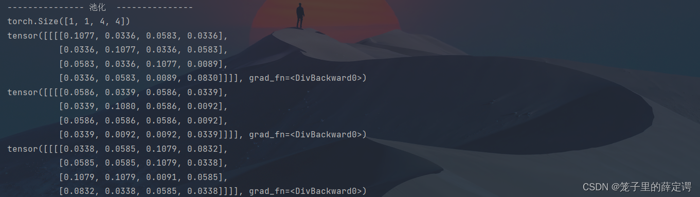
print("--------------- 池化 ---------------")
max_pool = nn.MaxPool2d(2, padding=0, stride=2) # Pooling
zeroPad = nn.ZeroPad2d(padding=(0, 1, 0, 1)) # pad 0 , Left Right Up Down
feature_map_pad_0_1 = zeroPad(feature_map1)
feature_pool_1 = max_pool(feature_map_pad_0_1)
feature_map_pad_0_2 = zeroPad(feature_map2)
feature_pool_2 = max_pool(feature_map_pad_0_2)
feature_map_pad_0_3 = zeroPad(feature_map3)
feature_pool_3 = max_pool(feature_map_pad_0_3)
print(feature_pool_1.size())
print(feature_pool_1 / 9)
print(feature_pool_2 / 9)
print(feature_pool_3 / 9)
img = feature_pool_1.data.squeeze().numpy() # 将输出转换为图片的格式
plt.figure(2, figsize=[50, 50], edgecolor='c', facecolor='c')
plt.subplot(331).set_title('特征图1补零结果')
plt.imshow(feature_map_pad_0_1.data.squeeze().numpy(), cmap=plt.cm.hot, vmin=-1, vmax=1)
plt.subplot(332).set_title('特征图2补零结果')
plt.imshow(feature_map_pad_0_2.data.squeeze().numpy(), cmap=plt.cm.hot, vmin=-1, vmax=1)
plt.subplot(333).set_title('特征图3补零结果')
plt.imshow(feature_map_pad_0_3.data.squeeze().numpy(), cmap=plt.cm.hot, vmin=-1, vmax=1)
plt.subplot(334).set_title('特征图1补零后池化结果')
plt.imshow(feature_pool_1.data.squeeze().numpy(), cmap=plt.cm.hot, vmin=-1, vmax=1)
plt.subplot(335).set_title('特征图2补零后池化结果')
plt.imshow(feature_pool_2.data.squeeze().numpy(), cmap=plt.cm.hot, vmin=-1, vmax=1)
plt.subplot(336).set_title('特征图3补零后池化结果')
plt.imshow(feature_pool_3.data.squeeze().numpy(), cmap=plt.cm.hot, vmin=-1, vmax=1)
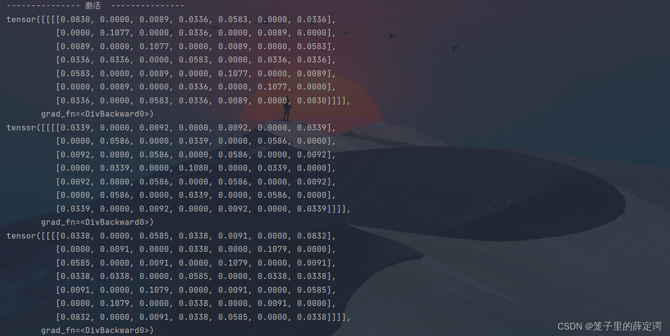
print("--------------- 激活 ---------------")
activation_function = nn.ReLU()
feature_relu1 = activation_function(feature_map1)
feature_relu2 = activation_function(feature_map2)
feature_relu3 = activation_function(feature_map3)
print(feature_relu1 / 9)
print(feature_relu2 / 9)
print(feature_relu3 / 9)
plt.subplot(337).set_title('特征图1池化后Relu激活结果')
plt.imshow(feature_relu1.data.squeeze().numpy(), cmap=plt.cm.hot, vmin=-1, vmax=1)
plt.subplot(338).set_title('特征图2池化后Relu激活结果')
plt.imshow(feature_relu2.data.squeeze().numpy(), cmap=plt.cm.hot, vmin=-1, vmax=1)
plt.subplot(339).set_title('特征图3池化后Relu激活结果')
plt.imshow(feature_relu3.data.squeeze().numpy(), cmap=plt.cm.hot, vmin=-1, vmax=1)
plt.show()
运行结果: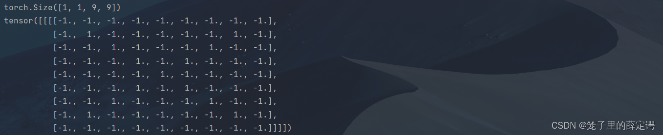
 可视化:
可视化: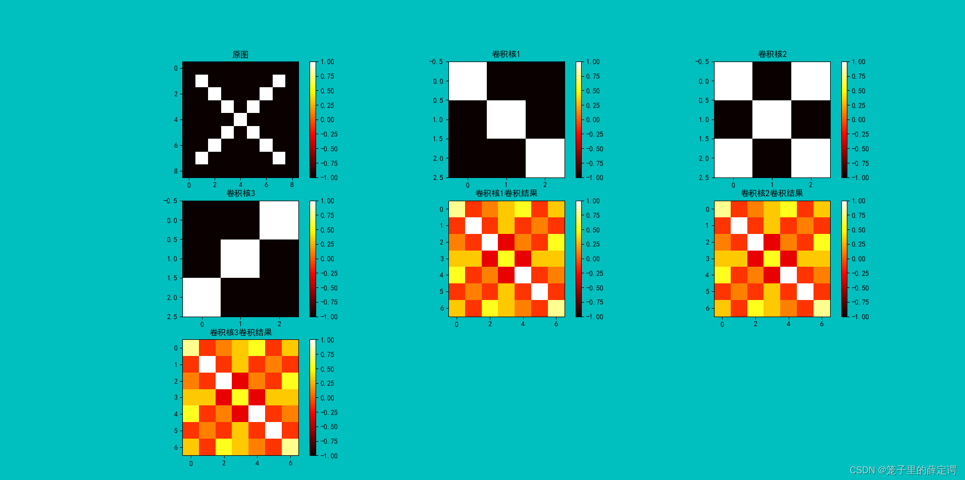
可视化: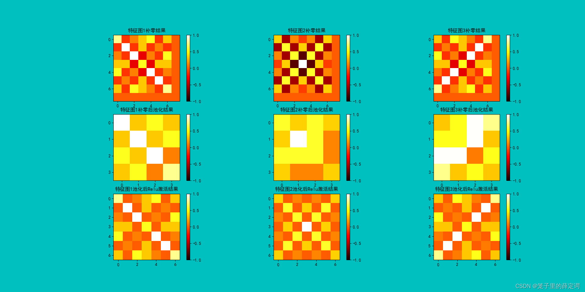
二、 基于CNN的XO识别
1. 数据集
XO数据集:
文件夹train_data:放置训练集 1700张图片,为850张X和850张O
文件夹test_data: 放置测试集 300张图片,为150张X和150张O
2. 构建模型
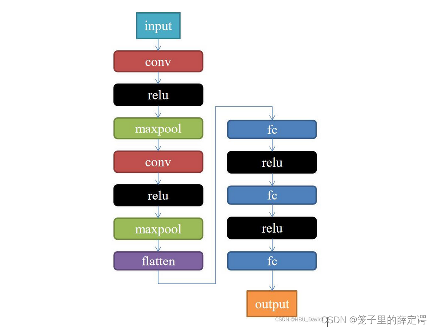
class Net(nn.Module):
    def __init__(self):
        super(Net, self).__init__()
        self.conv1 = nn.Conv2d(1, 9, 3)
        self.maxpool = nn.MaxPool2d(2, 2)
        self.conv2 = nn.Conv2d(9, 5, 3)

        self.relu = nn.ReLU()
        self.fc1 = nn.Linear(27 * 27 * 5, 1200)
        self.fc2 = nn.Linear(1200, 64)
        self.fc3 = nn.Linear(64, 2)

    def forward(self, x):
        x = self.maxpool(self.relu(self.conv1(x)))
        x = self.maxpool(self.relu(self.conv2(x)))
        x = x.view(-1, 27 * 27 * 5)
        x = self.relu(self.fc1(x))
        x = self.relu(self.fc2(x))
        x = self.fc3(x)
        return x
3.训练模型
注:因为有两千张图片,使用CPU速度较慢,对老师代码作了部分调整,使用GPU加速网络。
model = Net()

criterion = torch.nn.CrossEntropyLoss()  # 损失函数 交叉熵损失函数
optimizer = optim.SGD(model.parameters(), lr=0.1)  # 优化函数:随机梯度下降

use_gpu = torch.cuda.is_available()
if use_gpu:  # 有cuda
    print("use gpu for training")
    criterion = criterion.cuda()
    model = model.to('cuda')

epochs = 10
for epoch in range(epochs):
    running_loss = 0.0
    for i, data in enumerate(data_loader):
        images, label = data
        out = model(images.to('cuda')).to('cuda')
        loss = criterion(out, label.to('cuda'))

        optimizer.zero_grad()
        loss.backward()
        optimizer.step()

        running_loss += loss.item()
        if (i + 1) % 10 == 0:
            print('[%d  %5d]   loss: %.3f' % (epoch + 1, i + 1, running_loss / 100))
            running_loss = 0.0

print('finished train')
# 保存模型
torch.save(model, 'model_name.pth')  # 保存的是模型, 不止是w和b权重值
# torch.save(model.state_dict(), 'model_name1.pth')  # 保存的是w和b权重值
运行结果:

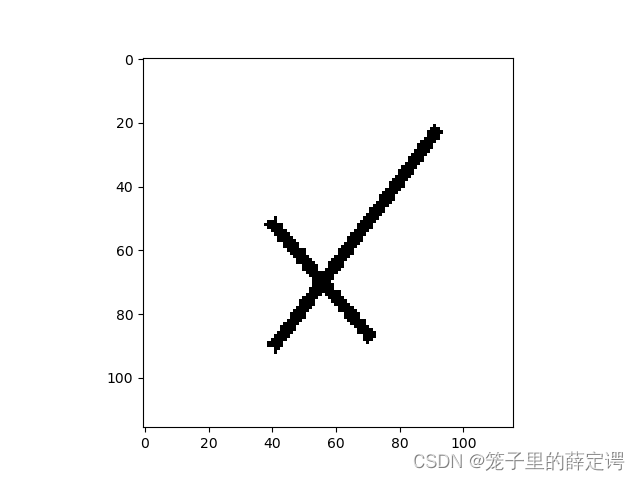
4.测试训练好的模型
# 读取模型
model_load = torch.load('model_name.pth')
# 读取一张图片 images[0],测试
print("labels[0] truth:\t", labels[0])
x = images[0]
x = x.reshape([1, x.shape[0], x.shape[1], x.shape[2]])
predicted = torch.max(model_load(x), 1)
print("labels[0] predict:\t", predicted.indices)

img = images[0].data.squeeze().numpy()  # 将输出转换为图片的格式
plt.imshow(img, cmap='gray')
plt.show()
运行结果:

5. 计算模型的准确率
model = Net()
model.load_state_dict(torch.load('model_name1.pth', map_location='cpu'))  # 导入网络的参数

correct = 0
total = 0
with torch.no_grad():  # 进行评测的时候网络不更新梯度
    for data in data_loader_test:  # 读取测试集
        images, labels = data
        outputs = model(images)
        _, predicted = torch.max(outputs.data, 1)  # 取出 最大值的索引 作为 分类结果
        total += labels.size(0)  # labels 的长度
        correct += (predicted == labels).sum().item()  # 预测正确的数目
print('Accuracy of the network on the  test images: %f %%' % (100. * correct / total))
运行结果:

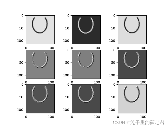
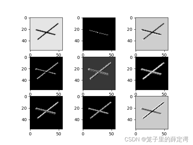
6.查看训练好的模型的特征图
import torch
import matplotlib.pyplot as plt
import numpy as np
from torchvision import transforms, datasets
import torch.nn as nn
from torch.utils.data import DataLoader

# 定义图像预处理过程
transforms = transforms.Compose([
    transforms.ToTensor(),  # 把图片进行归一化,并把数据转换成Tensor类型
    transforms.Grayscale(1)  # 把图片 转为灰度图
])
path = r'D:\project\DL\training_data_sm'
data_train = datasets.ImageFolder(path, transform=transforms)
data_loader = DataLoader(data_train, batch_size=64, shuffle=True)
for i, data in enumerate(data_loader):
    images, labels = data
    print(images.shape)
    print(labels.shape)
    break


class Net(nn.Module):
    def __init__(self):
        super(Net, self).__init__()
        self.conv1 = nn.Conv2d(1, 9, 3)  # in_channel , out_channel , kennel_size , stride
        self.maxpool = nn.MaxPool2d(2, 2)
        self.conv2 = nn.Conv2d(9, 5, 3)  # in_channel , out_channel , kennel_size , stride

        self.relu = nn.ReLU()
        self.fc1 = nn.Linear(27 * 27 * 5, 1200)  # full connect 1
        self.fc2 = nn.Linear(1200, 64)  # full connect 2
        self.fc3 = nn.Linear(64, 2)  # full connect 3

    def forward(self, x):
        outputs = []
        x = self.conv1(x)
        outputs.append(x)
        x = self.relu(x)
        outputs.append(x)
        x = self.maxpool(x)
        outputs.append(x)
        x = self.conv2(x)
        x = self.relu(x)
        x = self.maxpool(x)
        x = x.view(-1, 27 * 27 * 5)
        x = self.relu(self.fc1(x))
        x = self.relu(self.fc2(x))
        x = self.fc3(x)
        return outputs


# create model
model1 = Net()

# load model weights加载预训练权重
model_weight_path = "model_name1.pth"
model1.load_state_dict(torch.load(model_weight_path))

# 打印出模型的结构
print(model1)
x = images[0]
x = x.reshape([1, x.shape[0], x.shape[1], x.shape[2]])
# forward正向传播过程
out_put = model1(x)
for feature_map in out_put:
    im = np.squeeze(feature_map.detach().numpy())
    im = np.transpose(im, [1, 2, 0])
    print(im.shape)

    plt.figure()
    for i in range(9):
        ax = plt.subplot(3, 3, i + 1)
        plt.imshow(im[:, :, i], cmap='gray')
    plt.show()
运行结果:
网络结构: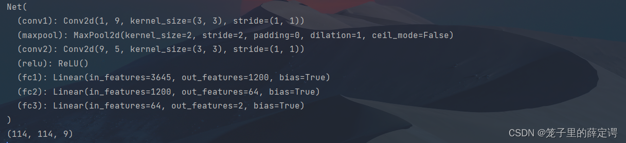

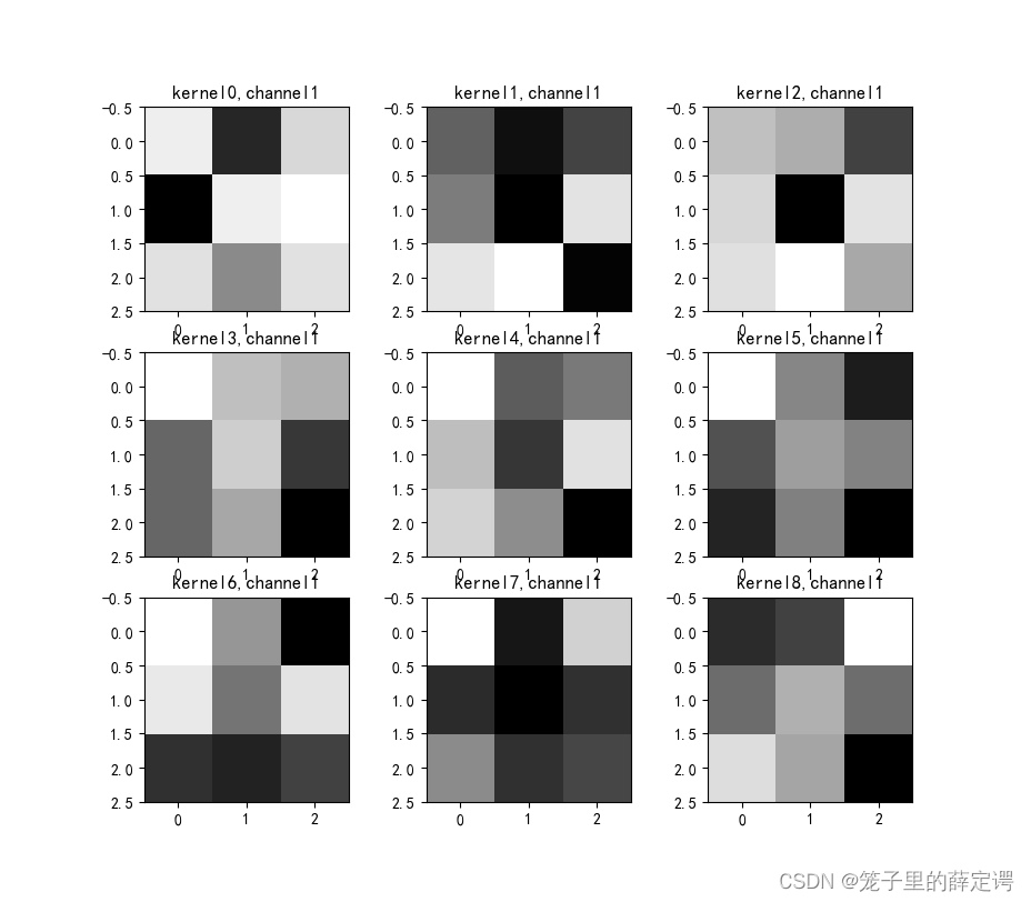
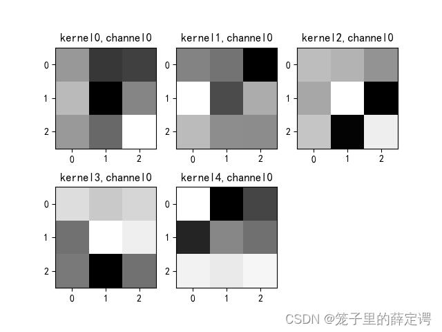
7. 查看训练好的模型的卷积核
import torch
import matplotlib.pyplot as plt
import numpy as np
from PIL import Image
from torchvision import transforms, datasets
import torch.nn as nn
from torch.utils.data import DataLoader

plt.rcParams['font.sans-serif'] = ['SimHei']  # 用来正常显示中文标签
plt.rcParams['axes.unicode_minus'] = False  # 用来正常显示负号 #有中文出现的情况,需要u'内容
#  定义图像预处理过程(要与网络模型训练过程中的预处理过程一致)
transforms = transforms.Compose([
    transforms.ToTensor(),  # 把图片进行归一化,并把数据转换成Tensor类型
    transforms.Grayscale(1)  # 把图片 转为灰度图
])
path =  r'D:\project\DL\training_data_sm'
data_train = datasets.ImageFolder(path, transform=transforms)
data_loader = DataLoader(data_train, batch_size=64, shuffle=True)
for i, data in enumerate(data_loader):
    images, labels = data
    break


class Net(nn.Module):
    def __init__(self):
        super(Net, self).__init__()
        self.conv1 = nn.Conv2d(1, 9, 3)  # in_channel , out_channel , kennel_size , stride
        self.maxpool = nn.MaxPool2d(2, 2)
        self.conv2 = nn.Conv2d(9, 5, 3)  # in_channel , out_channel , kennel_size , stride

        self.relu = nn.ReLU()
        self.fc1 = nn.Linear(27 * 27 * 5, 1200)  # full connect 1
        self.fc2 = nn.Linear(1200, 64)  # full connect 2
        self.fc3 = nn.Linear(64, 2)  # full connect 3

    def forward(self, x):
        outputs = []
        x = self.maxpool(self.relu(self.conv1(x)))
        # outputs.append(x)
        x = self.maxpool(self.relu(self.conv2(x)))
        outputs.append(x)
        x = x.view(-1, 27 * 27 * 5)
        x = self.relu(self.fc1(x))
        x = self.relu(self.fc2(x))
        x = self.fc3(x)
        return outputs


# create model
model1 = Net()

# load model weights加载预训练权重
model_weight_path = "model_name1.pth"
model1.load_state_dict(torch.load(model_weight_path))

x = images[0]
x = x.reshape([1, x.shape[0], x.shape[1], x.shape[2]])
# forward正向传播过程
out_put = model1(x)

weights_keys = model1.state_dict().keys()
for key in weights_keys:
    print("key :", key)
    # 卷积核通道排列顺序 [kernel_number, kernel_channel, kernel_height, kernel_width]
    if key == "conv1.weight":
        weight_t = model1.state_dict()[key].numpy()
        print("weight_t.shape", weight_t.shape)
        k = weight_t[:, 0, :, :]  # 获取第一个卷积核的信息参数
        # show 9 kernel ,1 channel
        plt.figure()

        for i in range(9):
            ax = plt.subplot(3, 3, i + 1)  # 参数意义:3:图片绘制行数,5:绘制图片列数,i+1:图的索引
            plt.imshow(k[i, :, :], cmap='gray')
            title_name = 'kernel' + str(i) + ',channel1'
            plt.title(title_name)
        plt.show()

    if key == "conv2.weight":
        weight_t = model1.state_dict()[key].numpy()
        print("weight_t.shape", weight_t.shape)
        k = weight_t[:, :, :, :]  # 获取第一个卷积核的信息参数
        print(k.shape)
        print(k)

        plt.figure()
        for c in range(9):
            channel = k[:, c, :, :]
            for i in range(5):
                ax = plt.subplot(2, 3, i + 1)  # 参数意义:3:图片绘制行数,5:绘制图片列数,i+1:图的索引
                plt.imshow(channel[i, :, :], cmap='gray')
                title_name = 'kernel' + str(i) + ',channel' + str(c)
                plt.title(title_name)
            plt.show()
运行结果:

8.源码
训练源码:
GPU版本(需要注意的模型保存部分,保存整个模型为:model_name.pth,只保存权重和偏置项为model_name1.pth):
import torch
from torchvision import transforms, datasets
import torch.nn as nn
from torch.utils.data import DataLoader
import torch.optim as optim
transforms = transforms.Compose([
transforms.ToTensor(), # 把图片进行归一化,并把数据转换成Tensor类型
transforms.Grayscale(1) # 把图片 转为灰度图
])
path = r'D:\project\DL\training_data_sm\train_data'
path_test = r'D:\project\DL\training_data_sm\test_data'
data_train = datasets.ImageFolder(path, transform=transforms)
data_test = datasets.ImageFolder(path_test, transform=transforms)
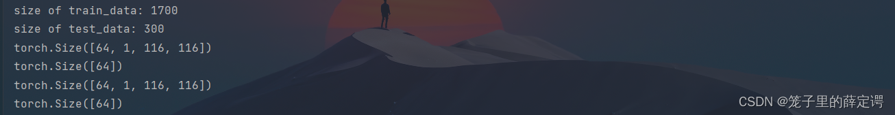
print("size of train_data:", len(data_train))
print("size of test_data:", len(data_test))
data_loader = DataLoader(data_train, batch_size=64, shuffle=True)
data_loader_test = DataLoader(data_test, batch_size=64, shuffle=True)
for i, data in enumerate(data_loader):
images, labels = data
print(images.shape)
print(labels.shape)
break
for i, data in enumerate(data_loader_test):
images, labels = data
print(images.shape)
print(labels.shape)
break
class Net(nn.Module):
def __init__(self):
super(Net, self).__init__()
self.conv1 = nn.Conv2d(1, 9, 3) # in_channel , out_channel , kennel_size , stride
self.maxpool = nn.MaxPool2d(2, 2)
self.conv2 = nn.Conv2d(9, 5, 3) # in_channel , out_channel , kennel_size , stride
self.relu = nn.ReLU()
self.fc1 = nn.Linear(27 * 27 * 5, 1200) # full connect 1
self.fc2 = nn.Linear(1200, 64) # full connect 2
self.fc3 = nn.Linear(64, 2) # full connect 3
def forward(self, x):
x = self.maxpool(self.relu(self.conv1(x)))
x = self.maxpool(self.relu(self.conv2(x)))
x = x.view(-1, 27 * 27 * 5)
x = self.relu(self.fc1(x))
x = self.relu(self.fc2(x))
x = self.fc3(x)
return x
model = Net()
criterion = torch.nn.CrossEntropyLoss() # 损失函数 交叉熵损失函数
optimizer = optim.SGD(model.parameters(), lr=0.1) # 优化函数:随机梯度下降
use_gpu = torch.cuda.is_available()
if use_gpu: # 有cuda
print("use gpu for training")
criterion = criterion.cuda()
model = model.to('cuda')
epochs = 10
for epoch in range(epochs):
running_loss = 0.0
for i, data in enumerate(data_loader):
images, label = data
out = model(images.to('cuda')).to('cuda')
loss = criterion(out, label.to('cuda'))
optimizer.zero_grad()
loss.backward()
optimizer.step()
running_loss += loss.item()
if (i + 1) % 10 == 0:
print('[%d %5d] loss: %.3f' % (epoch + 1, i + 1, running_loss / 100))
running_loss = 0.0
print('finished train')
# 保存模型
torch.save(model, 'model_name.pth') # 保存的是模型, 不止是w和b权重值
# torch.save(model.state_dict(), 'model_name1.pth') # 保存的是w和b权重值测试源码:
import torch
from torchvision import transforms, datasets
import torch.nn as nn
from torch.utils.data import DataLoader
import torch.optim as optim

transforms = transforms.Compose([
    transforms.ToTensor(),  # 把图片进行归一化,并把数据转换成Tensor类型
    transforms.Grayscale(1)  # 把图片 转为灰度图
])

path = r'D:\project\DL\training_data_sm\train_data'
path_test = r'D:\project\DL\training_data_sm\test_data'

data_train = datasets.ImageFolder(path, transform=transforms)
data_test = datasets.ImageFolder(path_test, transform=transforms)

print("size of train_data:", len(data_train))
print("size of test_data:", len(data_test))

data_loader = DataLoader(data_train, batch_size=64, shuffle=True)
data_loader_test = DataLoader(data_test, batch_size=64, shuffle=True)

for i, data in enumerate(data_loader):
    images, labels = data
    print(images.shape)
    print(labels.shape)
    break

for i, data in enumerate(data_loader_test):
    images, labels = data
    print(images.shape)
    print(labels.shape)
    break


class Net(nn.Module):
    def __init__(self):
        super(Net, self).__init__()
        self.conv1 = nn.Conv2d(1, 9, 3)  # in_channel , out_channel , kennel_size , stride
        self.maxpool = nn.MaxPool2d(2, 2)
        self.conv2 = nn.Conv2d(9, 5, 3)  # in_channel , out_channel , kennel_size , stride

        self.relu = nn.ReLU()
        self.fc1 = nn.Linear(27 * 27 * 5, 1200)  # full connect 1
        self.fc2 = nn.Linear(1200, 64)  # full connect 2
        self.fc3 = nn.Linear(64, 2)  # full connect 3

    def forward(self, x):
        x = self.maxpool(self.relu(self.conv1(x)))
        x = self.maxpool(self.relu(self.conv2(x)))
        x = x.view(-1, 27 * 27 * 5)
        x = self.relu(self.fc1(x))
        x = self.relu(self.fc2(x))
        x = self.fc3(x)
        return x
model = Net()
model.load_state_dict(torch.load('model_name1.pth', map_location='cpu'))  # 导入网络的参数

correct = 0
total = 0
with torch.no_grad():  # 进行评测的时候网络不更新梯度
    for data in data_loader_test:  # 读取测试集
        images, labels = data
        outputs = model(images)
        _, predicted = torch.max(outputs.data, 1)  # 取出 最大值的索引 作为 分类结果
        total += labels.size(0)  # labels 的长度
        correct += (predicted == labels).sum().item()  # 预测正确的数目
print('Accuracy of the network on the  test images: %f %%' % (100. * correct / total))
总结
1.第一部分作业为numpy手撸卷积-池化-激活和使用Pytorch包装好的卷积-池化-激活层,加深了一下这三层的印象,学习就是反复理解的过程。从运算结果来看二者相差不多,从可视化来看二者一模一样,因为这个小作业主要是观察每个阶段都干了什么,所以使用热力图进行了可视化。
2.第二部分作业主要是基于Pytorch搭建简单的卷积网络来实现XO识别,算是hello world的级别了,重点是刨析卷积过程,理解卷积过程中的卷积核由来(训练前和训练后)、特征图由来(卷积结果:相乘相加,有补零加上边缘的零算就行)以及卷积核参数的设置(现在基本可以口算卷积层各个阶段输出尺寸)。
3.这次作业使用的是老师的轮子,难度不大,就做了一下GPU网络加速以及可视化操作,卡在第二部分作业模型的保存和加载:
模型的加载和保存有两对搭档:
torch.save(model, 'model_name.pth') 和torch.load('model_name.pth');
torch.save(model.state_dict(), 'model_name1.pth') 和 model.load_state_dict(torch.load('model_name1.pth'))
后者更常用一些。
参考链接
【2021-2022 春学期】人工智能-作业6:CNN实现XO识别_HBU_David的博客-CSDN博客
【2021-2022 春学期】人工智能-作业5:卷积-池化-激活_HBU_David的博客-CSDN博客
torch — PyTorch 1.12 documentation


 226
226


 被折叠的 条评论
为什么被折叠?
被折叠的 条评论
为什么被折叠?
 到【灌水乐园】发言


