时间序列预测是能源、金融、交通、物流和云计算等各个行业的一项基本功能(Chen et al., 2012; Cirstea et al., 2022b; Ma et al., 2014; Zhu et al., 2023; Pan et al., 2023; Pedersen et al., 2020),也是其他时间序列分析的基础构建块,例如异常值检测 Campos et al. (2022);Kieu et al. (2022b)。 Transformer (Vaswani et al., 2017) 在序列建模中得到广泛应用,并在 CV 和 NLP 等各个领域取得了令人瞩目的成功 (Dosovitskiy et al., 2021; Brown et al., 2020),因此在时间序列领域受到越来越多的关注 (Wen et al., 2023; Wu et al., 2021; Chen et al., 2022; Liu et al., 2022c)。尽管性能不断提高,但最近的研究已经开始通过提出性能更好的更简单的线性模型来挑战现有的 Transformer 时间序列预测设计 (Zeng et al., 2023)。虽然 Transformer 在时间序列预测方面的能力仍然很有前景 (Nie et al., 2023),但它需要更好的设计和调整才能发挥其潜力。
为了进一步探索 Transformers 提取相关性以进行时间序列预测的能力,本文重点研究了使用 Transformer 架构增强多尺度建模的方面。两个主要挑战限制了 Transformers 中有效的多尺度建模。第一个挑战是多尺度建模的不完整性。从不同的时间分辨率查看数据会隐式地影响后续建模过程的尺度(Shabani et al., 2023)。然而,简单地改变时间分辨率不能明确有效地强调不同范围内的时间依赖性。相反,考虑不同的时间距离可以从不同范围建模依赖关系,例如全局和局部相关性(Li et al., 2019)。然而,全局和局部间隔的确切时间距离受数据划分的影响,从单一的时间分辨率角度来看这是不完整的。第二个挑战是固定的多尺度建模过程。虽然多尺度建模可以更完整地理解时间序列,但不同的序列根据其特定的时间特征和动态偏好不同的尺度。例如,比较图 1 中的两个序列,上面的序列显示出快速波动,这可能意味着需要更多地关注细粒度和短期特征。相反,下面的序列可能需要更多地关注粗粒度和长期建模。对所有数据进行固定的多尺度建模会阻碍对每个时间序列关键模式的把握,而手动调整数据集或每个时间序列的最佳尺度既耗时又难以解决。解决这两个挑战需要自适应多尺度建模,即从某些多个尺度自适应地对当前数据进行建模。
受上述对多尺度建模理解的启发,我们提出了具有自适应路径的多尺度 Transformers(Pathformer)用于时间序列预测。为了实现更完整的多尺度建模能力,我们提出了一个多尺度 Transformer 模块,统一了多尺度时间分辨率和时间距离。提出多尺度划分,将时间序列划分为不同大小的块,形成不同时间分辨率的视图。基于每个划分的块大小,提出了包含块间和块内注意的双重注意来捕获时间依赖性,其中块间注意捕获块之间的全局相关性,而块内注意捕获单个块内的局部细节。我们进一步提出了自适应路径来激活多尺度建模能力并赋予其自适应建模特性。在模型的每一层,多尺度路由器根据输入数据自适应地选择特定大小的块划分和 Transformer 中的后续双重注意,从而控制多尺度特征的提取。我们为路由器配备了趋势和季节性分解,以增强其掌握时间动态的能力。路由器与聚合器协同工作,通过加权聚合自适应地组合多尺度特征。逐层路由和聚合构成了整个 Transformer 中多尺度建模的自适应路径。据我们所知,这是第一项引入自适应多尺度建模进行时间序列预测的研究。具体来说,我们做出了以下贡献:
时间序列的多尺度建模。多尺度特征建模已被证明对于计算机视觉(Wang et al., 2021; Li et al., 2022b; Wang et al., 2022b)和多模态学习(Hu et al., 2020; Wang et al., 2022a)等领域的相关性学习和特征提取非常有效,但在时间序列预测中探索较少。N-HiTS(Challu et al., 2023)采用多速率数据采样和分层插值来对不同分辨率的特征进行建模。Pyraformer(Liu et al., 2022b)引入了金字塔注意力机制来提取不同时间分辨率的特征。Scaleformer(Shabani et al., 2023)提出了一个多尺度框架,需要在不同的时间分辨率下分配预测模型,这导致模型复杂度更高。与这些使用固定尺度、无法针对不同时间序列自适应地改变多尺度建模的方法不同,我们提出了一种具有自适应路径的多尺度 Transformer,可以根据不同的时间动态自适应地建模多尺度特征。
Inter-patch
attention establishes relationships between patches to capture global correlations. For
the patch-divided time series
X
∈
R
P
×
S
×
d
, we first perform feature embedding along the feature dimension from d
to
d
m
and then rearrange the data to combine the two dimensions of patch quantity S
and feature embedding
d
m
, resulting in
X
inter
∈
R
P
×
d'
m
, where
d
m
=
S
·
d
m
. After such embedding and rearranging process, the time steps within the same patch are combined, and thus we perform self-attention over X
inter
to model correlations between patches. Following the standard self-attention protocol, we obtain the query, key, and value through linear mapping on X
inter
, denoted as Q
inter
, K
inter
, V
inter
∈
R
P
×
d
′
m
. Then, we compute the attention
Attn
inter
, which involves interaction between patches and represents the global correlations of the time series:
块间注意力机制通过建立块间关系来捕捉全局相关性。对于
块划分后的时间序列 X ∈ R P ×S×d ,我们首先沿特征维度从 d 到 dm 进行特征嵌入,然后重新排列数据,将块数量 S 和特征嵌入 dm 两个维度结合起来,得到 Xinter ∈ R P ×d' m ,其中 d m = S · dm 。经过这样的嵌入和重新排列过程,同一个块内的时间步骤就被组合在一起了,因此我们在 Xinter 上进行自注意力来模拟块间的相关性。按照标准的自注意力协议,我们通过对 Xinter 的线性映射获得 query、key 和 value,记为 Qinter, Kinter, Vinter ∈ R P ×d′ m 。然后,我们计算注意力 Attninter ,它涉及块间的相互作用,表示时间序列的全局相关性:

To fuse global correlations and local details captured by dual attention, we rearrange the outputs
of intra-patch attention to
Attn
intra
∈
R
P
×
S
×
d
m
, performing linear transformations on the patch
size dimension from
1
to
S
, to combine time steps in each patch, and then add it with inter-patch
attention
Attn
inter
∈
R
P
×
S
×
d
m
to obtain the final output of dual attention
Attn
∈
R
P
×
S
×
d
m
.
Overall, the multi-scale division provides different views of the time series with different patch
sizes, and the changing patch sizes further influence the dual attention, which models temporal
dependencies from different distances guided by the patch division. These two components work
together to enable multiple scales of temporal modeling in the Transformer
为了融合双重注意捕获的全局相关性和局部细节,我们将块内注意的输出重新排列为 Attnintra ∈ R P ×S×dm,在块大小维度上执行从 1 到 S 的线性变换,以组合每个块中的时间步骤,然后将其与块间注意 Attninter ∈ R P ×S×dm 相加,以获得双重注意的最终输出 Attn ∈ R P ×S×dm。
总体而言,多尺度划分提供了具有不同块大小的时间序列的不同视图,而变化的块大小进一步影响双重注意,它在块划分的指导下从不同距离建模时间依赖性。这两个组件协同工作,使 Transformer 能够实现多尺度的时间建模.
3.2 ADAPTIVE PATHWAYS
The design of the multi-scale Transformer block equips the model with the capability of multiscale modeling. However, different series may prefer diverse scales, depending on their specific temporal characteristics and dynamics. Simply applying more scales may bring in redundant or
useless signals, and manually tuning the optimal scales for a dataset or each time series is time consuming or intractable. An ideal model needs to figure out such critical scales based on the input data for more effective modeling and better generalization of unseen data.
3.2 自适应路径
多尺度 Transformer 模块的设计使模型具备了多尺度建模的能力。然而,不同的序列可能偏好不同的尺度,这取决于它们特定的时间特征和动态。简单地应用更多尺度可能会带来冗余或无用的信号,而手动调整数据集或每个时间序列的最佳尺度是耗时的或难以解决的。理想的模型需要根据输入数据找出这些关键尺度,以便更有效地建模和更好地泛化未知数据。
Pathways and Mixture of Experts are used to achieve adaptive modeling (Dean, 2021; Shazeer et al., 2016). Based on these concepts, we propose adaptive pathways based on multi-scale Transformer to model adaptive multi-scale, depicted in Figure 2. It contains two main components: the multi-scale router and the multi-scale aggregator. The multi-scale router
selects specific sizes of patch division based on the input data, which activates specific parts in the Transformer and controls the extraction of multi-scale characteristics. The router works with the multi-scale aggregator
to combine these characteristics through weighted aggregation, obtaining the output of the Transformer block.
使用路径和专家混合来实现自适应建模(Dean,2021;Shazeer 等,2016)。基于这些概念,我们提出了基于多尺度 Transformer 的自适应路径来建模自适应多尺度,如图 2 所示。它包含两个主要组件:多尺度路由器和多尺度聚合器。多尺度路由器根据输入数据选择特定大小的 patch 划分,从而激活 Transformer 中的特定部分并控制多尺度特征的提取。路由器与多尺度聚合器协同工作,通过加权聚合将这些特征组合起来,得到 Transformer 块的输出。
Multi-Scale Router.
The multi-scale router enables data-adaptive routing in the multi-scale Transformer, which selects the optimal sizes for patch division and thus controls the process of multi-scale modeling. Since the optimal or critical scales for each time series can be impacted by its complex inherent characteristics and dynamic patterns, like the periodicity and trend, we introduce a temporal decomposition module in the router that encompasses both seasonality and trend decomposition
to extract periodicity and trend patterns, as illustrated in Figure 3(b).
多尺度路由器。多尺度路由器可在多尺度 Transformer 中实现数据自适应路由,从而选择最佳的块划分尺寸,控制多尺度建模过程。由于每个时间序列的最优或临界尺度可能受其复杂的固有特性和动态模式(如周期性和趋势)的影响,我们在路由器中引入了一个时间分解模块,该模块同时包含季节性和趋势分解,以提取周期性和趋势模式,如图 3(b) 所示。
Seasonality decomposition
involves transforming the time series from the temporal domain into the frequency domain to extract the periodic patterns. We utilize the Discern Fourier Transform (DFT
) (Cooley & Tukey, 1965), denoted as DFT(
·
)
, to decompose the input
X
into Fourier basis and select the K
f
basis with the largest amplitudes to keep the sparsity of frequency domain. Then, we obtain the periodic patterns X
sea
through an inverse DFT, denoted as
IDFT(
·
)
. The process is as follows:
季节性分解涉及将时间序列从时间域转换为频域以提取周期模式。我们利用离散傅里叶变换(DFT)(Cooley & Tukey,1965),表示为DFT(·),将输入X分解为傅里叶基,并选择幅度最大的Kf基以保持频域的稀疏性。然后,我们通过逆DFT(表示为IDFT(·))获得周期模式Xsea。过程如下:
where
Φ
and
A
represent the phase and amplitude of each frequency from
DFT(X)
,
{
f
1
, . . . , f
K
f
}
represents the frequencies with the top
K
f
amplitudes.
Trend decomposition
uses different kernels of average pooling for moving averages to extract trend patterns based on the remaining part after the seasonality decomposition X
rem
= X
−
X
sea
. For the results obtained from different kernels, a weighted operation is applied to obtain the representation of the trend component:
其中 Φ 和 A 表示来自 DFT(X) 的每个频率的相位和幅度,{f1, . . . , fKf }
表示幅度最大的 Kf 个频率。趋势分解使用不同的平均池化核对移动平均,根据季节性分解后的剩余部分 Xrem = X − Xsea 提取趋势模式。对于从不同核获得的结果,应用加权运算以获得趋势成分的表示:

where
Avgpool(
·
)
kernel
i
is the pooling function with the
i
-th kernel,
N
corresponds to the number
of kernels,
Softmax(
L
(
·
))
controls the weights for the results from different kenerls. We add the
seasonality pattern and trend pattern with the original input
X
, and then perform a linear mapping
Linear(
·
)
to transform and merge them along the temporal dimension to get
X
trans
∈
R
d
.
其中 Avgpool(·)kerneli 为第 i 个核的池化函数,N 对应核的数量,Softmax(L(·)) 控制不同核的结果的权重。我们将季节性模式和趋势模式与原始输入 X 相加,然后进行线性映射 Linear(·) 沿时间维度进行变换和合并,得到 Xtrans ∈ R d 。
Based on the results
X
trans
from temporal decomposition, the router employs a routing function
to generate the pathway weights, which determines the patch sizes to choose for the current data. To avoid consistently selecting a few patch sizes, causing the corresponding scales to be repeatedly updated while neglecting other potentially useful scales in the multi-scale Transformer, we introduce noise terms to add randomness in the weight generation process. The whole process of generating pathway weights is as follows:
基于时间分解的结果 Xtrans,路由器使用路由函数来生成路径权重,从而确定当前数据要选择的补丁大小。为了避免始终选择少数补丁大小,导致相应的尺度重复更新,同时忽略多尺度 Transformer 中其他可能有用的尺度,我们引入了噪声项以在权重生成过程中增加随机性。生成路径权重的整个过程如下:
where
R
(
·
)
represents the whole routing function,
W
r
and
W
noise
∈
R
d
×
M
are learnable parameters for weight generation, with d
denoting the feature dimension of
X
trans
and
M
denoting the number of patch sizes. To introduce sparsity in the routing and encourage the selection of critical scales, we perform topK
selection on the pathway weights, keeping the top
K
pathway weights and setting the rest weights as 0
, and denote the final result as
R
¯(X
trans
)
.
其中 R(·) 表示整个路由函数,Wr 和 Wnoise ∈ R d×M 是权重生成的可学习参数,d 表示 Xtrans 的特征维度,M 表示块大小的数量。为了在路由中引入稀疏性并鼓励选择关键尺度,我们对路径权重进行 topK 选择,保留前 K 个路径权重并将其余权重设置为 0,并将最终结果表示为 R¯(Xtrans)。
Multi-Scale Aggregator.
Each dimension of the generated pathway weights
R
¯(X
trans
)
∈
R
M
correspond to a patch size in the multi-scale Transformer, with R
¯(X
trans
)
i
>
0
indicating performing this size S
i
of patch division and the dual attention and
R
¯(X
trans
)
i
= 0
indicating ignoring this patch size for the current data. Let X
i
out
denote the output of the multi-scale Transformer with the patch size S
i
, due to the varying temporal dimensions produced by different patch sizes, the aggregator first perform a transformation function T
i
(
·
)
to align the temporal dimension from different scales. Then, the aggregator performs weighted aggregation for the multi-scale outputs based on the pathway weights to get the final output of this AMS block:

I
(
R
¯(X
trans
)
i
>
0)
is the indicator function which outputs
1
when
R
¯(X
trans
)
i
>
0
, and other
wise outputs
0
, indicating that only the top
K
patch sizes and the corresponding outputs from the
Transformer are considered or needed during aggregation.
I(R¯(Xtrans)i > 0) 是指示函数,当 R¯(Xtrans)i > 0 时输出 1,否则输出 0,表示在聚合过程中仅考虑或需要前 K 个补丁大小和 Transformer 的相应输出。
4 EXPERIMENTS
4.1 TIME SERIES FORECASTING
Datasets.
We conduct experiments on nine real-world datasets to assess the performance of Pathformer, encompassing a range of domains, including electricity transportation, weather forecasting, and cloud computing. These datasets include ETT (ETTh1, ETTh2, ETTm1, ETTm2), Weather, Electricity, Traffic, ILI, and Cloud Cluster (Cluster-A, Cluster-B, Cluster-C).
4 实验
4.1 时间序列预测
数据集。我们对九个真实数据集进行了实验,以评估 Pathformer 的性能,涵盖了一系列领域,包括电力运输、天气预报和云计算。这些数据集包括 ETT(ETTh1、ETTh2、ETTm1、ETTm2)、天气、电力、交通、ILI 和云集群(Cluster-A、Cluster-B、Cluster-C)。
Implementation Details.
Pathformer utilizes the Adam optimizer (Kingma & Ba, 2015) with a
learning rate set at
10
−
3
. The default loss function employed is L1 Loss, and we implement early
stopping within 10 epochs during the training process. All experiments are conducted using PyTorch and executed on an NVIDIA A800 80GB GPU. Pathformer is composed of 3 Adaptive Multi-Scale Blocks (AMS Blocks). Each AMS Block contains 4 different patch sizes. These patch sizes are selected from a pool of commonly used options, namely {
2
,
3
,
6
,
12
,
16
,
24
,
32
}
.
实施细节。Pathformer 使用 Adam 优化器 (Kingma & Ba, 2015),学习率设置为 10−3。使用的默认损失函数是 L1 损失,我们在训练过程中在 10 个时期内实现提前停止。所有实验均使用 PyTorch 进行,并在 NVIDIA A800 80GB GPU 上执行。Pathformer 由 3 个自适应多尺度块 (AMS 块) 组成。每个 AMS 块包含 4 种不同的补丁大小。这些补丁大小是从常用选项池中选择的,即 {2, 3, 6, 12, 16, 24, 32}。
Main Results.
Table 1 shows the prediction results of multivariable time series forecasting, where Pathformer stands out with the best performance in 81 cases and the second-best in 5 cases out of the overall 88 cases. Compared with the second-best baseline, PatchTST, Pathformer demonstrates a significant improvement, with an impressive 8.1% reduction in MSE and a 6.4% reduction in MAE. Compared with the strong linear models NLinear, Pathformer also outperforms them comprehensively, especially on large datasets such as Electricity and Traffic. This demonstrates the potential of Transformer architecture for time series forecasting. Compared with the multi-scale models Pyraformer and Scaleformer, Pathformer exhibits good performance improvements, with a substantial 36.4% reduction in MSE and a 19.1% reduction in MAE. This illustrates that the proposed comprehensive modeling from both temporal resolution and temporal distance with adaptive pathways is more effective for multi-scale modeling.
主要结果。表 1 显示了多变量时间序列预测的预测结果,其中 Pathformer 在 81 个案例中表现最佳,在 88 个案例中的 5 个案例中表现第二。与第二好的基线 PatchTST 相比,Pathformer 表现出显着的改进,MSE 降低了 8.1%,MAE 降低了 6.4%。与强线性模型 NLinear 相比,Pathformer 也全面胜过它们,尤其是在电力和交通等大型数据集上。这证明了 Transformer 架构在时间序列预测方面的潜力。与多尺度模型 Pyraformer 和 Scaleformer 相比,Pathformer 表现出良好的性能改进,MSE 降低了 36.4%,MAE 降低了 19.1%。这说明,所提出的具有自适应路径的时间分辨率和时间距离综合建模对于多尺度建模更有效。
4.2 TRANSFER LEARNING
Experimental Setting.
To assess the transferability of Pathformer, we benchmark it against three
baselines: PatchTST, FEDformer, and Autoformer, devising two distinct transfer experiments. In the context of evaluating transferability across different datasets, models initially undergo pre-training on the ETTh1 and ETTm1. Subsequently, we fine-tune them using the ETTh2 and ETTm2. For assessing transferability towards future data, models are pre-trained on the first 70% of the training data sourced from three clusters: Cluster-A, Cluster-B, and Cluster-C. This pre-training is followed by fine-tuning the remaining 30% of the training data specific to each cluster. In terms of methodology for baselines, we explore two approaches: direct prediction (zero-shot) and full-tuning. Deviating from these approaches, Pathformer integrates a part-tuning strategy. In this approach, specific parameters, like those of the router network, undergo fine-tuning, resulting in a significant reduction in computational resource demands.
4.2 迁移学习
实验设置。为了评估 Pathformer 的可迁移性,我们将其与三个
基线进行对比:PatchTST、FEDformer 和 Autoformer,设计了两个不同的迁移实验。在评估不同数据集之间的可迁移性时,模型首先在 ETTh1 和 ETTm1 上进行预训练。随后,我们使用 ETTh2 和 ETTm2 对它们进行微调。为了评估未来数据的可迁移性,模型在来自三个集群的前 70% 的训练数据上进行预训练:Cluster-A、Cluster-B 和 Cluster-C。在进行预训练之后,对每个集群剩余的 30% 的训练数据进行微调。在基线方法方面,我们探索了两种方法:直接预测(零样本)和完全调整。与这些方法不同,Pathformer 集成了部分调整策略。在这种方法中,特定参数(例如路由器网络的参数)会经过微调,从而显著减少计算资源需求。
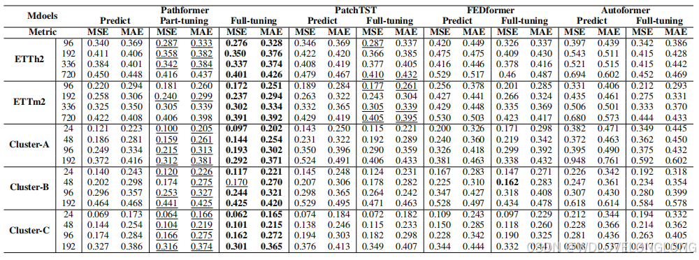
Transfer Learning Results.
Table 2 presents the outcomes of our transfer learning evaluation.
Across both direct prediction and full-tuning methods, Pathformer surpasses the baseline models,
highlighting its enhanced generalization and transferability. One of the key strengths of Pathformer lies in its adaptive capacity to select varying scales for different temporal dynamics. This adaptability allows it to effectively capture complex temporal patterns present in diverse datasets, consequently demonstrating superior generalization and transferability. Part-tuning is a lightweight fine-tuning method that demands fewer computational resources and reduces training time on average by 52%
, while still achieving prediction accuracy nearly comparable to Pathformer full-tuning. Moreover, it outperforms the full-tuning of other baseline models on the majority of datasets. This demonstrates that Pathformer can provide effective lightweight transfer learning for time series forecasting.
迁移学习结果。表 2 展示了我们对迁移学习的评估结果。
在直接预测和完全调整方法中,Pathformer 都超越了基线模型,突出了其增强的泛化和可迁移性。Pathformer 的主要优势之一在于它能够根据不同的时间动态选择不同的尺度。这种适应性使其能够有效地捕捉不同数据集中存在的复杂时间模式,从而展示出卓越的泛化和可迁移性。部分调整是一种轻量级的微调方法,它需要更少的计算资源,平均减少 52% 的训练时间,同时仍能实现与 Pathformer 完全调整几乎相当的预测精度。此外,它在大多数数据集上的表现都优于其他基线模型的完全调整。这表明 Pathformer 可以为时间序列预测提供有效的轻量级迁移学习。
Table 1: Multivariate time series forecasting results. The input length
H
= 96
(
H
= 36
for ILI).
The best results are highlighted in bold, and the second-best results are underlined.
表 1:多元时间序列预测结果。输入长度 H = 96(ILI 为 H = 36)。
最佳结果以粗体突出显示,次佳结果以下划线突出显示。
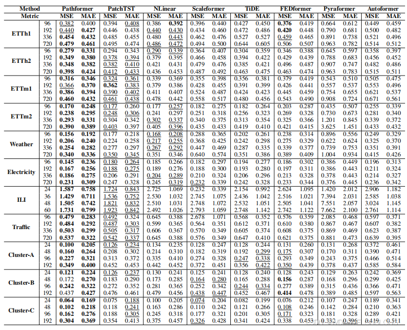
Table 2: Transfer Learning results. The best results are in bold, and the second results are underlined.
表 2:迁移学习结果。最佳结果以粗体显示,第二个结果以下划线显示。
4.3 ABLATION STUDIES
To ascertain the impact of different modules within Pathformer, we perform ablation studies focusing on inter-patch attention, intra-patch attention, time series decomposition, and Pathways. The W/O Pathways configuration entails using all patch sizes from the patch size pool for every dataset, eliminating adaptive selection. Table 3 illustrates the unique impact of each module. The influence of Pathways is significant; omitting them results in a marked decrease in prediction accuracy. This emphasizes the criticality of optimizing the mix of patch sizes to extract multi-scale characteristics, thus markedly improving the model’s prediction accuracy. Regarding efficiency, intra-patch attention is notably adept at discerning local patterns, contrasting with inter-patch attention which primarily captures wider global patterns. The time series decomposition module decomposes trend and periodic patterns to improve the ability to capture the temporal dynamics of its input, assisting in the identification of appropriate patch sizes for combination.
4.3 消融研究
为了确定 Pathformer 中不同模块的影响,我们进行了消融研究,重点关注块间注意、块内注意、时间序列分解和路径。W/O 路径配置需要对每个数据集使用块大小池中的所有块大小,从而消除自适应选择。表 3 说明了每个模块的独特影响。路径的影响很大;省略它们会导致预测精度明显下降。这强调了优化块大小组合以提取多尺度特征的重要性,从而显著提高模型的预测精度。就效率而言,块内注意特别擅长辨别局部模式,而块间注意主要捕捉更广泛的全局模式。时间序列分解模块分解趋势和周期模式,以提高捕捉其输入的时间动态的能力,帮助识别适合组合的块大小。
Table 3: Ablation study. W/O Inter, W/O Intra, W/O Decompose represent removing the inter-patch attention, intra-patch attention, and time series decomposition, respectively.
表 3:消融研究。W/O Inter、W/O Intra、W/O Decompose 分别代表去除块间注意力、块内注意力和时间序列分解。
Table 4: Parameter sensitivity study. The prediction accuracy varies with
K.
表4:参数敏感性研究。预测精度随K值变化。
Varying the Number of Adaptively Selected Patch Sizes.
Pathformer adaptively selects the top
K
patch sizes for combination, adjusting to different time series samples. We evaluate the influence of different K
values on prediction accuracy in Table 4. Our findings show that
K
= 2
and
K
= 3 yield better results than K
= 1
and
K
= 4
, highlighting the advantage of adaptively modeling
critical multi-scale characteristics for improved accuracy. Additionally, distinct time series samples
benefit from feature extraction using varied patch sizes, but not all patch sizes are equally effective.
改变自适应选择的补丁大小的数量。Pathformer 自适应地选择前 K 个补丁大小进行组合,以适应不同的时间序列样本。我们在表 4 中评估了不同 K 值对预测精度的影响。我们的研究结果表明,K = 2 和 K = 3 产生的结果比 K = 1 和 K = 4 更好,突出了自适应建模关键多尺度特征以提高精度的优势。此外,不同的时间序列样本受益于使用不同补丁大小的特征提取,但并非所有补丁大小都同样有效。
Visualization of Pathways Weights.
We show three samples and depict their average Pathways weights for each patch size in Figure 4. Our observations reveal that the samples possess unique Pathways weight distributions. Both Samples 1 and 2, which demonstrate longer seasonality and similar trend patterns, show similar visualized Pathways weights. This manifests in the higher weights they attribute to the larger patch sizes. On the other hand, Sample 3, which is characterized by its shorter seasonality pattern, aligns with higher weights for the smaller patch sizes. These observations underscore Pathformer’s adaptability, emphasizing its ability to discern and apply the optimal patch size combinations for the diverse seasonality and trend patterns across samples.
路径权重的可视化。我们展示了三个样本,并在图 4 中描绘了每个斑块大小的平均路径权重。我们的观察表明,这些样本具有独特的路径权重分布。样本 1 和 2 都表现出较长的季节性和相似的趋势模式,并显示出相似的可视化路径权重。这表现在它们赋予较大斑块大小的权重较高。另一方面,样本 3 的特点是其较短的季节性模式,与较小斑块大小的权重较高一致。这些观察结果强调了 Pathformer 的适应性,强调了它能够辨别和应用最佳斑块大小组合,以适应样本间不同的季节性和趋势模式。
Figure 4: The average pathways weights of different patch sizes for the Weather.
B
1
,
B
2
, and
B
3
denote distinct AMS (Adaptive Multi-Scale) blocks, while
S
1
,
S
2
,
S
3
, and
S
4
represent varying
patch sizes within each AMS block, with patch size decreasing sequentially.
图 4:天气中不同斑块大小的平均路径权重。B1、B2 和 B3表示不同的 AMS(自适应多尺度)块,而 S1、S2、S3 和 S4 表示每个 AMS 块内不同的斑块大小,斑块大小依次减小。
5 CONCLUSION
In this paper, we propose Pathformer, a Multi-Scale Transformer with Adaptive Pathways for time
series forecasting. It integrates multi-scale temporal resolutions and temporal distances by introducing patch division with multiple patch sizes and dual attention on the divided patches, enabling the comprehensive modeling of multi-scale characteristics. Furthermore, adaptive pathways dynamically select and aggregate scale-specific characteristics based on the different temporal dynamics. These innovative mechanisms collectively empower Pathformer to achieve outstanding prediction performance and demonstrate strong generalization capability on several forecasting tasks.
5 结论
在本文中,我们提出了 Pathformer,一种用于时间序列预测的具有自适应路径的多尺度 Transformer。它通过引入具有多种块大小的块划分和对划分的块的双重注意,将多尺度时间分辨率和时间距离集成在一起,从而实现多尺度特征的综合建模。此外,自适应路径根据不同的时间动态动态选择和聚合特定于尺度的特征。这些创新机制共同使 Pathformer 能够实现出色的预测性能,并在多个预测任务上表现出强大的泛化能力。
A
CKNOWLEDGMENTS
This work was supported by National Natural Science Foundation of China (62372179) and Alibaba Innovative Research Program
致谢
本研究得到国家自然科学基金(62372179)和阿里巴巴创新研究计划的支持
二、MMFNET: MULTI-SCALE FREQUENCY MASKING NEURAL NETWORK FOR MULTIVARIATE TIME SERIES FORECASTING
MMFNET: 用于多变量时间序列预测的多尺度频率掩蔽神经网络
Aitian Ma, Dongsheng Luo, Mo Sha Knight Foundation School of Computing and Information Sciences Florida International University Miami, FL, USA
{
aima,dluo,msha
}
@fiu.edu
摘要:
Long-term Time Series Forecasting (LTSF) is critical for numerous real-world applications, such as electricity consumption planning, financial forecasting, and disease propagation analysis. LTSF requires capturing long-range dependencies between inputs and outputs, which poses significant challenges due to complex temporal dynamics and high computational demands. While linear models reduce model complexity by employing frequency domain decomposition, current approaches often assume stationarity and filter out high-frequency components that may contain crucial short-term fluctuations. In this paper, we introduce MMFNet, a novel model designed to enhance long-term multivariate forecasting by leveraging a multi-scale masked frequency decomposition approach. MMFNet captures fine, intermediate, and coarse-grained temporal patterns by converting time series into frequency segments at varying scales while employing a learnable mask to filter out irrelevant components adaptively. Extensive experimentation with benchmark datasets shows that MMFNet not only addresses the limitations of the existing methods but also consistently achieves good performance. Specifically, MMFNet achieves up to 6.
0%
reductions in the Mean Squared Error (MSE) compared to state-of-the-art models designed for multivariate forecasting tasks.
长期时间序列预测 (LTSF) 对于许多实际应用至关重要,例如电力消耗规划、财务预测和疾病传播分析。LTSF 需要捕获输入和输出之间的长期依赖关系,这由于复杂的时间动态和高计算需求而带来了重大挑战。虽然线性模型通过采用频域分解来降低模型复杂性,但当前方法通常假设平稳性并滤除可能包含关键短期波动的高频分量。在本文中,我们介绍了 MMFNet,这是一种新颖的模型,旨在通过利用多尺度掩蔽频率分解方法来增强长期多元预测。MMFNet 通过将时间序列转换为不同尺度的频率段来捕获细粒度、中粒度和粗粒度的时间模式,同时采用可学习的掩码自适应地滤除不相关的成分。对基准数据集的大量实验表明,MMFNet 不仅解决了现有方法的局限性,而且始终如一地实现了良好的性能。具体来说,与针对多元预测任务设计的最先进的模型相比,MMFNet 将均方误差 (MSE) 降低了 6.0%。
1 I
NTRODUCTION
Time series forecasting is pivotal in a wide range of domains, such as environmental monitoring (Bhandari et al., 2017), electrical grid management (Zufferey et al., 2017), financial analysis (Sezer et al., 2020), and healthcare (Zeroual et al., 2020). Accurate long-term forecasting is
essential for informed decision-making and strategic planning. Traditional methods, such as autoregressive (AR) models (Nassar et al., 2004), exponential smoothing (Hyndman & Athanasopoulos, 2008), and structural time series models (Harvey, 1989), have provided a robust foundation for time series analysis by leveraging historical data to predict future values. However, real-world systems frequently exhibit complex, non-stationary behavior, with time series characterized by intricate patterns such as trends, fluctuations, and cycles. Those complexities pose significant challenges to achieving accurate forecasts (Makridakis et al., 1998; Box et al., 2015).
1 引言
时间序列预测在环境监测(Bhandari 等人,2017 年)、电网管理(Zufferey 等人,2017 年)、财务分析(Sezer 等人,2020 年)和医疗保健(Zeroual 等人,2020 年)等众多领域都至关重要。准确的长期预测对于明智的决策和战略规划至关重要。传统方法,例如自回归 (AR) 模型(Nassar 等人,2004 年)、指数平滑(Hyndman & Athanasopoulos,2008 年)和结构时间序列模型(Harvey,1989 年),通过利用历史数据预测未来值,为时间序列分析提供了坚实的基础。然而,现实世界的系统经常表现出复杂的非平稳行为,时间序列具有复杂的模式,例如趋势、波动和周期。这些复杂性对实现准确预测构成了重大挑战(Makridakis 等人,1998 年;Box 等人,2015 年)。
Long-term Time Series Forecasting (LTSF) has seen significant advancements in recent years, driven by the development of sophisticated models, such as Transformer-based models (Zhou et al., 2021; Wu et al., 2021; Nie et al., 2024) and linear models (Zeng et al., 2023; Xu et al., 2024; Lin et al., 2024). Transformer-based architectures have demonstrated exceptional capacity in capturing complex temporal patterns by effectively modeling long-range dependencies through self-attention mechanisms at the cost of heavy computation workload, particularly when facing large-scale time series data, which significantly limits their practicality in real-time applications.
近年来,长期时间序列预测 (LTSF) 取得了重大进展,这得益于基于 Transformer 的模型 (Zhou et al., 2021; Wu et al., 2021; Nie et al., 2024) 和线性模型 (Zeng et al., 2023; Xu et al., 2024; Lin et al., 2024) 等复杂模型的发展。基于 Transformer 的架构通过自注意力机制有效地对长距离依赖关系进行建模,表现出捕捉复杂时间模式的卓越能力,但计算工作量很大,尤其是在面对大规模时间序列数据时,这大大限制了它们在实时应用中的实用性。
In contrast, the linear models provide a lightweight alternative for real-time forecasting. In particular, FITS demonstrates superior predictive performance across a wide range of scenarios with only 10K
parameters by utilizing a single-scale frequency domain decomposition method combined witha low-pass filter employing a fixed cutoff frequency (Xu et al., 2024). While single-scale frequency domain decomposition offers a global perspective of time series data in the frequency domain, it lacks the ability to localize specific frequency components within the sequence. Furthermore, such methods assume that frequency components remain constant throughout the entire sequence, thereby failing to account for the non-stationary behavior frequently observed in real-world time series. Additionally, the low-pass filter employed by FITS may inadvertently smooth out crucial short-term fluctuations necessary for accurate predictions. The fixed cutoff frequency of the low-pass filter may not be universally optimal for diverse time series datasets, further limiting its adaptability.
相比之下,线性模型为实时预测提供了一种轻量级的替代方案。特别是,FITS 通过利用单尺度频域分解方法结合采用固定截止频率的低通滤波器,在仅 10K 个参数的广泛场景中表现出卓越的预测性能(Xu 等人,2024 年)。虽然单尺度频域分解提供了频域中时间序列数据的全局视角,但它缺乏在序列内定位特定频率分量的能力。此外,这类方法假设频率分量在整个序列中保持不变,因此无法解释现实世界时间序列中经常观察到的非平稳行为。此外,FITS 使用的低通滤波器可能会无意中平滑准确预测所需的关键短期波动。低通滤波器的固定截止频率可能不是针对各种时间序列数据集的普遍最优的,从而进一步限制了其适应性。
In this paper, we present MMFNet, a novel model designed to enhance LTSF through a multiscale masked frequency decomposition approach. MMFNet captures fine, intermediate, and coarsegrained patterns in the frequency domain by segmenting the time series at multiple scales. At each scale, MMFNet employs a learnable mask that adaptively filters out irrelevant frequency components based on the segment’s spectral characteristics. MMFNet offers two key advantages: (i) the multiscale frequency decomposition enables MMFNet to effectively capture both short-term fluctuations and broader trends in the data, and (ii) the learnable frequency mask adaptively filters irrelevant frequency components, allowing the model to focus on the most informative signals. These features make MMFNet well-suited to capturing both short-term and long-term dependencies in complex time series, positioning it as an effective solution for various LTSF tasks.
在本文中,我们介绍了 MMFNet,这是一种通过多尺度掩蔽频率分解方法增强 LTSF 的新模型。MMFNet 通过在多个尺度上分割时间序列来捕获频域中的细、中和粗粒度模式。在每个尺度上,MMFNet 都采用可学习的掩码,根据片段的频谱特性自适应地滤除不相关的频率成分。MMFNet 具有两个关键优势:(i) 多尺度频率分解使 MMFNet 能够有效捕获数据中的短期波动和更广泛的趋势,(ii) 可学习的频率掩码自适应地过滤不相关的频率成分,使模型能够专注于最具信息量的信号。这些特性使 MMFNet 非常适合捕获复杂时间序列中的短期和长期依赖关系,使其成为各种 LTSF 任务的有效解决方案。
In summary, the contributions of this paper are as follows:
• To our knowledge, MMFNet is the first model that employs multi-scale frequency domain decomposition to capture the dynamic variations in the frequency domain;
• MMFNet introduces a novel learnable masking mechanism that adaptively filters out irrelevant
frequency components;
• Extensive experiments show that MMFNet consistently achieves good performance in a variety of multivariate time series forecasting tasks, with up to a 6
.
0%
reduction in the Mean Squared Error (MSE) compared to the existing models.
综上所述,本文的贡献如下:
• 据我们所知,MMFNet 是第一个采用多尺度频域分解来捕捉频域动态变化的模型;
• MMFNet 引入了一种新颖的可学习掩蔽机制,可以自适应地滤除不相关的频率成分;
• 大量实验表明,MMFNet 在各种多元时间序列预测任务中始终保持良好的性能,与现有模型相比,均方误差 (MSE) 降低了 6.0%。
2 P
RELIMINARIES
Long-term Time Series Forecasting. LTSF involves predicting future values over an extended time horizon based on previously observed multivariate time series data. The LTSF problem can be formulated as:
where
x
t
−
L
+1:
t
∈
R
L
×
C
denotes the historical observation window, and
x
ˆ
t
+1:
t
+
H
∈
R
H
×
C
represents the predicted future values. In this formulation, L
is the length of the historical window,
H
is the forecast horizon, and
C
denotes the number of features or channels. As the forecast horizon H
increases, the models face challenges to accurately capture both long-term and short-term dependencies within the time series.
2 准备工作
长期时间序列预测。LTSF 涉及根据先前观察到的多变量时间序列数据预测长期范围内的未来值。LTSF 问题可以表述为:
其中 xt−L+1:t ∈ R L×C 表示历史观察窗口,xˆt+1:t+H ∈ R H×C 表示预测的未来值。在这个公式中,L 是历史窗口的长度,H 是预测范围,C 表示特征或通道的数量。随着预测范围 H 的增加,模型面临着准确捕捉时间序列中长期和短期依赖关系的挑战。
Single-Scale Frequency Transformation (SFT).
SFT refers to the process of converting the timedomain data into the frequency domain at a single, global scale without segmenting the time series. Such a transformation is typically performed using methods, such as the Fast Fourier Transform (FFT), which efficiently computes the Discrete Fourier Transform (DFT). SFT decomposes the entire signal into sinusoidal components, enabling the analysis of its frequency content. Each frequency component can be expressed as:
单尺度频率变换 (SFT)。
SFT 是指将时域数据以单一、全局尺度转换为频域的过程,而无需对时间序列进行分段。这种变换通常使用快速傅里叶变换 (FFT) 等方法执行,这些方法可以高效计算离散傅里叶变换 (DFT)。SFT 将整个信号分解为正弦分量,从而可以分析其频率内容。每个频率分量可以表示为:
where
|
X
k
|
represents the amplitude and
ϕ
k
the phase of the
k
-th frequency component. While
the frequency decomposition provides valuable insights into periodic patterns and trends, traditional approaches assume stationarity and operate on a global scale, limiting their capacity to capture the complex, non-stationary characteristics frequently observed in real-world time series. Current frequency-based LTSF models, such as FITS (Xu et al., 2024), implement this method by performing frequency domain interpolation at a single scale, which can be formulated as:
其中 |Xk| 表示振幅,ϕk 表示第 k 个频率分量的相位。虽然
频率分解提供了对周期模式和趋势的宝贵见解,但传统方法假设平稳性并在全球范围内运行,限制了它们捕捉现实世界时间序列中经常观察到的复杂非平稳特征的能力。当前基于频率的 LTSF 模型,例如 FITS(Xu 等人,2024 年),通过在单一尺度上执行频域插值来实现此方法,可以将其表述为:

where
F
denotes the Fourier transform, and
g
represents the filtering operation applied uniformly
across the signal. Although SFT is capable of capturing broad temporal patterns, such as long-term trends through low-pass filtering or short-term fluctuations through high-pass filtering, its global application treats the entire signal uniformly. This uniform treatment may result in the loss of important local temporal variations and non-stationary behaviors occurring at different scales.
其中 F 表示傅立叶变换,g 表示对信号均匀应用的滤波操作。虽然 SFT 能够捕捉广泛的时间模式,例如通过低通滤波捕捉长期趋势或通过高通滤波捕捉短期波动,但其全局应用会均匀处理整个信号。这种均匀处理可能会导致重要的局部时间变化和不同尺度上发生的非平稳行为的丢失。
3 M
ETHOD
3.1 O
VERVIEW
To overcome the limitations of SFT, we propose the Multi-scale Masked Frequency Transformation (MMFT). MMFT performs frequency decomposition across multiple temporal scales, enabling the model to capture both global and local temporal patterns. Formally, the MMFT problem can be expressed as:
3 方法
3.1 概述
为了克服 SFT 的局限性,我们提出了多尺度掩蔽频率变换 (MMFT)。MMFT 在多个时间尺度上执行频率分解,使模型能够捕捉全局和局部时间模式。正式地,MMFT 问题可以表示为:
where F
s
denotes the frequency transformation at scale
s
, and
h
represents the aggregation and
filtering operation applied to the learnable frequency masks at various scales. Unlike SFT, which
applies a single transformation to the entire time series, MMFT divides the signal into multiple
scales, each subjected to frequency decomposition. At each scale, a learnable frequency mask is applied to retain the most informative frequency components while selectively discarding noise. This multi-scale approach allows the model to adapt to non-stationary signals, capturing complex dependencies that span different temporal ranges. By leveraging frequency decomposition at multiple scales and applying adaptive masks, MMFT enhances long-term forecasting accuracy by focusing on both short-term fluctuations and long-term trends within the data. This method increases the model’s flexibility and robustness, particularly for non-stationary and multivariate time series. Further analysis of the differences between SFT and MMFT can be found in Appendix B.
其中 Fs 表示尺度 s 的频率变换,h 表示对不同尺度的可学习频率掩码应用的聚合和过滤操作。与对整个时间序列应用单一变换的 SFT 不同,MMFT 将信号划分为多个尺度,每个尺度都经过频率分解。在每个尺度上,应用可学习的频率掩码以保留最具信息量的频率分量,同时有选择地丢弃噪声。这种多尺度方法使模型能够适应非平稳信号,捕获跨越不同时间范围的复杂依赖关系。通过利用多个尺度的频率分解和应用自适应掩码,MMFT 可以关注数据中的短期波动和长期趋势,从而提高长期预测的准确性。这种方法提高了模型的灵活性和稳健性,特别是对于非平稳和多变量时间序列。有关 SFT 和 MMFT 之间差异的进一步分析,请参见附录 B。
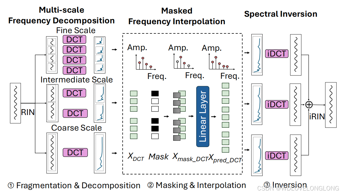
Figure 1: MMFNet Architecture. MMFNet consists of the following key components:
⃝
1 The input time series is first normalized to have zero mean using Reversible Instance-wise Normalization (RIN) (Lai et al., 2021). The multi-scale frequency decomposition process then divides the time
series instance
X
into fine, intermediate, and coarse-scale segments, which are subsequently transformed into the frequency domain via the Discrete Cosine Transform (DCT). ⃝
2 A learnable mask is applied to the frequency segments, followed by a linear layer that predicts the transformed frequency components. ⃝
3 Finally, the predicted frequency segments from each scale are transformed back into the time domain, merged, and denormalized using inverse RIN (iRIN).
图 1:MMFNet 架构。MMFNet 由以下关键组件组成:⃝1 首先使用可逆实例归一化 (RIN) (Lai et al., 2021) 将输入时间序列归一化为零均值。然后,多尺度频率分解过程将时间序列实例 X 划分为细尺度、中尺度和粗尺度段,随后通过离散余弦变换 (DCT) 将其变换到频域。⃝2 将可学习的掩码应用于频率段,然后是预测变换后的频率分量的线性层。⃝3 最后,将每个尺度的预测频率段变换回时间域,合并并使用逆 RIN (iRIN) 进行反归一化。
MMFNet enhances time series forecasting by incorporating the proposed MMFT method to capture intricate frequency features across different scales. The overall architecture of MMFNet is
depicted in Figure 1. The model comprises three key components: Multi-scale Frequency Decomposition, Masked Frequency Interpolation, and Spectral Inversion. Multi-scale Frequency Decomposition normalizes the input time series, divides it into segments of varying scales, and transforms these segments into the frequency domain using the DCT. Masked Frequency Interpolation applies a self-adaptive, learnable mask to filter out irrelevant frequency components, followed by a linear transformation of the filtered frequency domain segments. Finally, Spectral Inversion converts the processed frequency components back into the time domain via the Inverse Discrete Cosine Transform (iDCT) (Ahmed et al., 1974). The outputs from different scales are then aggregated, resulting in a refined signal that preserves the essential characteristics of the original input.
MMFNet 通过结合所提出的 MMFT 方法来捕获不同尺度上的复杂频率特征,从而增强了时间序列预测。MMFNet 的整体架构如图 1 所示。该模型包括三个关键组件:多尺度频率分解、掩蔽频率插值和频谱反演。多尺度频率分解对输入时间序列进行归一化,将其划分为不同尺度的段,并使用 DCT 将这些段变换到频域。掩蔽频率插值应用自适应、可学习的掩码来滤除不相关的频率分量,然后对滤波后的频域段进行线性变换。最后,频谱反演通过逆离散余弦变换 (iDCT) (Ahmed 等,1974) 将处理后的频率分量转换回时域。然后聚合来自不同尺度的输出,从而产生保留原始输入基本特征的精细信号。
3.2 M
ULTI
-
SCALE
F
REQUENCY
D
ECOMPOSITION
The core concept of Multi-scale Frequency Decomposition lies in applying frequency domain transformations to time series sequences at multiple scales. This approach enables the model to capture both global patterns and fine-grained temporal dynamics by analyzing the data across various segment levels. Multi-scale Frequency Decomposition consists of two fundamental steps: fragmentation and decomposition. Details about the overall workflow can be seen in Appendix A.1
3.2 多尺度频率分解
多尺度频率分解的核心概念在于将频域变换应用于多尺度的时间序列。这种方法使模型能够通过分析各个分段级别的数据来捕捉全局模式和细粒度的时间动态。多尺度频率分解包括两个基本步骤:碎片化和分解。有关整体工作流程的详细信息,请参见附录 A.1
Fragmentation.
This step decomposes the time series data into segments of varying lengths to capture features across multiple scales. Specifically, the input sequence X
is first normalized using RIN (Lai et al., 2021) and then partitioned into three sets of segments: fine-scale, intermediate-scale, and coarse-scale segments. Fine-scale segments (X
f ine
) consist of shorter segments that capture detailed, high-frequency components of the time series, enabling the detection of intricate patterns and anomalies that may be missed in longer segments. Intermediate-scale segments (X
intermediate
) are of moderate length and are designed to capture intermediate-level patterns and trends, striking a balance between the fine and coarse segments. Coarse-scale segments (X
coarse
) comprise longer segments that capture broader, low-frequency trends and overarching patterns within the data. This multi-scale fragmentation allows the model to effectively capture and leverage patterns across different temporal scales.
碎片化。
此步骤将时间序列数据分解为不同长度的段,以捕获跨多个尺度的特征。具体而言,首先使用 RIN(Lai 等人,2021)对输入序列 X 进行归一化,然后将其划分为三组段:细尺度、中等尺度和粗尺度段。细尺度段 (Xf ine) 由较短的段组成,可捕获时间序列的详细高频分量,从而能够检测较长段中可能遗漏的复杂模式和异常。中等尺度段 (Xintermediate) 长度适中,旨在捕获中等级别的模式和趋势,在细尺度段和粗尺度段之间取得平衡。粗尺度段 (Xcoarse) 由较长的段组成,可捕获数据中更广泛的低频趋势和总体模式。这种多尺度碎片化使模型能够有效地捕获和利用跨不同时间尺度的模式。
Decomposition.
This step converts the multi-scale time-domain segments into their corresponding frequency components to capture frequency patterns across various temporal scales. For each segment, the DCT is applied to extract frequency domain representations. Specifically, the fine-scale
segments in
X
f ine
are transformed into
X
DCT f ine
, the intermediate-scale segments in
X
intermediate are converted into X
DCT intermediate
, and the coarse-scale segments in
X
coarse
are transformed into
X
DCT coarse
.
分解。
此步骤将多尺度时域段转换为其相应的频率分量,以捕获跨各种时间尺度的频率模式。对于每个段,应用 DCT 来提取频域表示。具体而言,Xf ine 中的细尺度段转换为 XDCT f ine ,Xintermediate 中的中等尺度段转换为 XDCT middle ,Xcoarse 中的粗尺度段转换为 XDCT coarse 。
The DCT for each segment is computed using the following formula:每个段的 DCT 使用以下公式计算:
where
x
n
represents the time-domain signal values,
N
is the segment length, and
k
denotes the
frequency component. The resulting coefficients
X
k
represent the frequency components of the
segment. This transformation enables MMFNet to capture and analyze patterns at multiple temporal scales in the frequency domain, thereby enhancing its ability to recognize and interpret complex patterns in time series data.
其中 xn 表示时域信号值,N 表示段长度,k 表示频率分量。所得系数 Xk 表示段的频率分量。这种转换使 MMFNet 能够在频域中捕获和分析多个时间尺度上的模式,从而增强其识别和解释时间序列数据中复杂模式的能力。
3.3 M
ASKED
F
REQUENCY
I
NTERPOLATION
Masked Frequency Interpolation leverages a learnable mask to adaptively filter frequency components across different scales in the frequency domain, followed by reconstruction through a linear layer neural network. This approach enables the model to learn and apply scale-specific filtering strategies tailored to diverse datasets. The process consists of two primary steps: Masking and Interpolation.
3.3 掩蔽频率插值
掩蔽频率插值利用可学习的掩蔽来自适应地过滤频域中不同尺度的频率分量,然后通过线性层神经网络进行重建。这种方法使模型能够学习和应用针对不同数据集量身定制的尺度特定过滤策略。该过程包括两个主要步骤:掩蔽和插值。
Masking.
Traditional methods often employ fixed low-pass filters with a predefined cutoff frequency to filter frequency components. These approaches assume that certain frequencies are universally important or irrelevant across the entire time series, an assumption that may not hold for
non-stationary data where the relevance of frequency components varies over time. Moreover, overfiltering can lead to the loss of critical details, resulting in oversimplified representations and diminished model performance in tasks such as forecasting and signal analysis. To address these
limitations, MMFNet employs an adaptive masking technique to capture dynamic behaviors in the
frequency domain. Given the frequency segments
X
DCT
, a learnable mask is generated to adaptively filter the frequency components. The mask adjusts the significance of different frequency components by attenuating or emphasizing them based on their relevance to the task. This filtering process is applied via element-wise multiplication, represented as:
where
⊙
denotes element-wise multiplication,
M
represents the learnable mask, and
X
mask DCT
is the resulting masked frequency representation. During training, the mask is iteratively updated
based on the loss function, allowing MMFNet to focus on the most relevant aspects of the frequency domain representation. This adaptive mechanism improves the model’s capacity to capture meaningful patterns while minimizing the influence of irrelevant or noisy information.
掩蔽。
传统方法通常采用具有预定义截止频率的固定低通滤波器来过滤频率分量。这些方法假设某些频率在整个时间序列中普遍重要或不相关,这一假设可能不适用于非平稳数据,因为非平稳数据中频率分量的相关性随时间而变化。此外,过度过滤可能导致关键细节的丢失,从而导致表示过于简单,模型在预测和信号分析等任务中的性能下降。为了解决这些限制,MMFNet 采用自适应掩蔽技术来捕获频域中的动态行为。给定频率段 XDCT ,生成可学习的掩码以自适应地过滤频率分量。掩码通过根据它们与任务的相关性来衰减或强调不同频率分量来调整它们的重要性。此过滤过程通过元素乘法应用,表示为:
其中 ⊙ 表示元素乘法,M 表示可学习掩码,Xmask DCT是得到的掩码频率表示。在训练过程中,掩码会根据损失函数进行迭代更新,从而使 MMFNet 能够专注于频域表示中最相关的方面。这种自适应机制提高了模型捕获有意义模式的能力,同时最大限度地减少了无关或嘈杂信息的影响。
Interpolation.
In this step, the masked frequency segments
X
mask DCT
are transformed into predicted frequency domain segments X
pred DCT
through a linear layer. This linear transformation
maps the filtered frequency components to the target frequency representations aligned with the
model’s forecasting objectives. Specifically, a fully connected (dense) layer is applied to the masked frequency components, and this operation can be expressed as:
插值。
在此步骤中,通过线性层将屏蔽频率段 Xmask DCT 转换为预测频域段 Xpred DCT。此线性变换
将滤波后的频率分量映射到与模型的预测目标一致的目标频率表示。具体而言,对屏蔽频率分量应用全连接(密集)层,此操作可表示为:
where
W
denotes the weight matrix of the linear layer, and
b
is the bias term. The linear layer
is designed to learn a projection that aligns the filtered frequency components with the target prediction space. This transformation further refines the frequency domain information, producing
X
pred DCT
, which is essential for reconstructing accurate time-domain predictions. By leveraging the refined frequency information and reducing the influence of irrelevant frequency components, this step improves the overall prediction accuracy.
其中 W 表示线性层的权重矩阵,b 表示偏置项。线性层旨在学习将滤波后的频率分量与目标预测空间对齐的投影。此变换进一步细化了频域信息,产生了Xpred DCT ,这对于重建准确的时域预测至关重要。通过利用细化的频率信息并减少不相关频率分量的影响,此步骤可提高整体预测准确性。
3.4 S
PECTRAL
I
NVERSION
The final process, Spectral Inversion, transforms the interpolated frequency components back into the time domain using the iDCT, reversing the earlier DCT process. The iDCT is applied individually to the predicted frequency domain segments X
pred f ine DCT
,
X
pred intermediate DCT
, and
X
pred coarse DCT
. The iDCT for a segment is given by the following formula:
3.4 频谱反转
最后一个过程是频谱反转,它使用 iDCT 将插值频率分量转换回时域,从而逆转了之前的 DCT 过程。iDCT 分别应用于预测的频域段 Xpred 精细 DCT 、Xpred 中间 DCT 和 Xpred 粗 DCT 。段的 iDCT 由以下公式给出:
where
x
n
represents the time-domain signal values,
X
k
are the frequency components, and
N
denotes the segment length. This equation reconstructs the time-domain signal by summing the contributions of each frequency component (Davis & Marsaglia, 1984).
其中 xn 表示时域信号值,Xk 为频率分量,N 表示段长度。该方程通过对每个频率分量的贡献求和来重建时域信号(Davis & Marsaglia,1984)。
Once the iDCT is performed separately for each scale, the resulting time-domain signals are combined. This integration step merges the multi-scale frequency information by combining the outputs from the fine, intermediate, and coarse scales. The final reconstructed signal preserves the key characteristics of the original input while incorporating the enhanced interpolation achieved through the masked frequency filtering.
一旦对每个尺度分别执行 iDCT,就会将得到的时域信号组合起来。此集成步骤通过组合细尺度、中尺度和粗尺度的输出来合并多尺度频率信息。最终的重建信号保留了原始输入的关键特性,同时结合了通过屏蔽频率滤波实现的增强插值。
4 E
XPERIMENT
In this section, we evaluate MMFNet with several LTSF benchmark datasets across a range of forecast horizons. We also conduct ablation studies to assess the impact of MMFT and our frequency masking techniques. Finally, we evaluate MMFNet’s performance in ultra-long-term forecasting scenarios.
4 实验
在本节中,我们使用多个 LTSF 基准数据集在一系列预测范围内评估 MMFNet。我们还进行了消融研究,以评估 MMFT 和我们的频率掩蔽技术的影响。最后,我们评估了 MMFNet 在超长期预测场景中的表现。
4.1 E
XPERIMENTAL
S
ETUP
Datasets.
We perform experiments with seven widely-used LTSF datasets: ETTh1, ETTh2, ETTm1, ETTm2, Weather, Electricity, and Traffic. More details on those datasets can be found in Appendix A.2.
Baselines.
We compare MMFNet against several state-of-the-art models, including FEDformer (Zhou et al., 2022b), TimesNet (Wu et al., 2023), TimeMixer (Wang et al., 2024), and PatchTST (Nie et al., 2024). In addition, we compare MMFNet against several lightweight models, including DLinear (Zeng et al., 2023), FITS (Xu et al., 2024), and SparseTSF (Lin et al., 2024). More details on our baseline models can be found in Appendix A.3.
Environment.
All experiments are implemented using PyTorch (Paszke et al., 2019) and run on a single NVIDIA GeForce RTX 4090 GPU with 24
GB of memory
4.1 实验设置
数据集。
我们使用七个广泛使用的 LTSF 数据集进行实验:ETTh1、ETTh2、ETTm1、ETTm2、天气、电力和交通。有关这些数据集的更多详细信息,请参阅附录 A.2。
基线。
我们将 MMFNet 与几种最先进的模型进行了比较,包括 FEDformer(Zhou et al.,2022b)、TimesNet(Wu et al.,2023)、TimeMixer(Wang et al.,2024)和 PatchTST(Nie et al.,2024)。此外,我们将 MMFNet 与几种轻量级模型进行了比较,包括 DLinear(Zeng et al.,2023)、FITS(Xu et al.,2024)和 SparseTSF(Lin et al.,2024)。有关我们的基线模型的更多详细信息,请参阅附录 A.3。
环境。
所有实验均使用 PyTorch(Paszke 等人,2019 年)实现,并在具有 24GB 内存的单个 NVIDIA GeForce RTX 4090 GPU 上运行
4.2 P
ERFORMANCE ON
LTSF B
ENCHMARKS
Table 1: Multivariate LTSF MSE results on ETT, Weather, Electricity, and Traffic. The best result
is emphasized in
bold
, while the second-best is underlined. “Imp.” represents the improvement
between MMFNet and either the best or second-best result, with a higher “Imp.” indicating greater improvement.
4.2 LTSF 基准测试中的表现
表 1:ETT、天气、电力和交通的多元 LTSF MSE 结果。最佳结果
以粗体突出显示,而第二佳结果则用下划线表示。“Imp.”表示 MMFNet 与最佳或第二佳结果之间的改进,其中“Imp.”越高,表示改进越大。
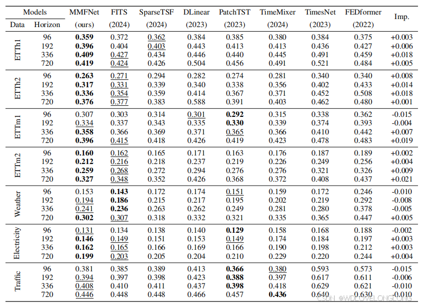
The experimental results offer several key insights into MMFNet’s performance across a range of
datasets and forecast horizons. As Table 1 shows, MMFNet demonstrates superior performance
on the ETT dataset and consistently achieves the best results even at extended forecasting horizons. Additionally, it maintains strong performance across a range of channel numbers and sampling rates.
实验结果为 MMFNet 在一系列数据集和预测范围内的性能提供了几个关键见解。如表 1 所示,MMFNet 在 ETT 数据集上表现出色,即使在扩展的预测范围内也能始终取得最佳结果。此外,它在一系列通道数和采样率上都保持了强劲的性能。
Performance on the ETT Dataset.
As Table 1 shows, MMFNet consistently outperforms other models across all forecast horizons on the ETTh1, ETTh2, and ETTm2 datasets. For example,on ETTh1, compared with other baseline models, MMFNet achieves the best MSE results of 0
.
359
, 0.
396
,
0
.
409
, and
0
.
419
at forecast horizons of
96
,
192
,
336
, and
720
, respectively. Moreover, it demonstrates a 4.
2%
MSE reduction (+0.018) at the forecast horizon of
336
on ETTh1 and a
5
.
1% MSE reduction (+0.018) at the forecast horizon of 336
on ETTh2. This consistent performance highlights MMFNet’s ability to effectively capture both short-term fluctuations and long-term dependencies in time series data, positioning it as a versatile model for a wide variety of LTSF tasks.
ETT 数据集上的表现。
如表 1 所示,在 ETTh1、ETTh2 和 ETTm2 数据集上的所有预测范围内,MMFNet 的表现始终优于其他模型。例如,在 ETTh1 上,与其他基线模型相比,MMFNet 在预测范围 96、192、336 和 720 时分别实现了 0.359、0.396、0.409 和 0.419 的最佳 MSE 结果。此外,它在 ETTh1 的预测范围 336 上显示出 4.2% 的 MSE 降低(+0.018),在 ETTh2 的预测范围 336 上显示出 5.1% 的 MSE 降低(+0.018)。这种一致的性能凸显了 MMFNet 有效捕捉时间序列数据中的短期波动和长期依赖性的能力,使其成为各种 LTSF 任务的多功能模型。
Performance at the Extended Horizon.
As Table 1 shows, at the extended forecast horizon of 720, MMFNet consistently achieves the highest predictive accuracy across all datasets, except for Traffic where it ranks second. Notably, MMFNet demonstrates significant improvements over baseline models, achieving MSE reductions of 4
.
6%
(
+0
.
019
) on ETTm1 and
6
.
0%
(
+0
.
021
) on ETTm2 at forecast horizon 720
compared to the second-best models. These results highlight the robustness of MMFNet in addressing long-term forecasting tasks.
扩展范围内的性能。
如表 1 所示,在扩展预测范围 720 内,MMFNet 在所有数据集中始终保持最高的预测准确率,但 Traffic 除外,它排名第二。值得注意的是,MMFNet 比基线模型有显著改进,与排名第二的模型相比,在预测范围 720 内,ETTm1 上的 MSE 降低了 4.6% (+0.019),ETTm2 上的 MSE 降低了 6.0% (+0.021)。这些结果凸显了 MMFNet 在解决长期预测任务方面的稳健性。
Performance in Low-Channel, Low-Sampling Rate Scenarios.
As Table 1 shows, in scenarios involving datasets with fewer channels (7 channels) and lower sampling rates (1-hour intervals), such as in the ETTh1 and ETTh2 datasets, linear models like FITS, SparseTSF, and DLinear exhibit strong performance. For example, on ETTh2, FITS achieves the MSE results of 0
.
271
,
0
.
331
, 0.
354
, and
0
.
377
at forecast horizons of
96
,
192
,
336
, and
720
, respectively. MMFNet continues to surpass these models on ETTh2 by achieving the MSE results of 0
.
263
,
0
.
317
,
0
.
336
, and
0
.
376
at forecast horizons of 96
,
192
,
336
, and
720
, respectively. This suggests that multi-scale frequency decomposition methods are particularly well-suited for datasets with fewer channels and broader time intervals between measurements.
低通道、低采样率场景下的性能。
如表 1 所示,在涉及通道较少(7 个通道)和采样率较低(1 小时间隔)的数据集场景中,例如在 ETTh1 和 ETTh2 数据集中,FITS、SparseTSF 和 DLinear 等线性模型表现出色。例如,在 ETTh2 上,FITS 在预测范围 96、192、336 和 720 时分别实现了 0.271、0.331、0.354 和 0.377 的 MSE 结果。MMFNet 在 ETTh2 上继续超越这些模型,在预测范围 96、192、336 和 720 时分别实现了 0.263、0.317、0.336 和 0.376 的 MSE 结果。这表明多尺度频率分解方法特别适合通道较少、测量时间间隔较长的数据集。
Performance in High-Channel Scenarios.
As Table 1 shows, for datasets with larger numbers of channels, such as Electricity (321
channels,
1
-hour sampling rate) and Traffic (
862
channels,
1
- hour sampling rate), MMFNet and FITS consistently demonstrate strong performance. Despite the increased complexity that arises from higher channel counts. For example, on Electricity, MMFnet achieves the best MSE results of 0
.
146
,
0
.
162
, and
0
.
199
at forecast horizons of
192
,
336
, and
720
, respectively. MMFNet’s multi-scale frequency decomposition enables it to effectively model complex temporal dependencies while maintaining high predictive accuracy. While PatchTST performs better on the traffic dataset, it leverages a patching transformer mechanism rather than a purely linear frequency-based approach, distinguishing it from MMFNet and FITS in terms of the model
architecture. This further indicates that more sophisticated decomposition methods are required for lightweight models to handle high-channel scenarios effectively.
高通道场景下的性能。
如表 1 所示,对于具有更多通道的数据集,例如电力(321 个通道,1 小时采样率)和交通(862 个通道,1 小时采样率),MMFNet 和 FITS 始终表现出强劲的性能。尽管更高的通道数会增加复杂性。例如,在电力方面,MMFnet 在预测范围分别为 192、336 和 720 时分别实现了 0.146、0.162 和 0.199 的最佳 MSE 结果。MMFNet 的多尺度频率分解使其能够有效地模拟复杂的时间依赖性,同时保持较高的预测准确性。虽然 PatchTST 在交通数据集上表现更好,但它利用了修补变压器机制,而不是纯线性基于频率的方法,在模型架构方面将其与 MMFNet 和 FITS 区分开来。这进一步表明,轻量级模型需要更复杂的分解方法来有效处理高通道场景。
Performance in High-Sampling Rate Scenarios.
As Table 1 shows, for datasets with higher sampling rates, such as Weather (21
channels,
10
-minute sampling rate), ETTm1 and ETTm2 (
7
channels, 15
-minute sampling rate), MMFNet and FITS consistently demonstrate strong performance. For example, on ETTm2, MMFnet achieves the best MSE results of 0
.
160
,
0
.
212
,
0
.
259
, and
0
.
327 at forecast horizons of 96
,
192
,
336
, and
720
, respectively. Despite the increased complexity that arises from a faster sampling rate, MMFNet’s multi-scale frequency decomposition enables it to effectively model complex temporal dependencies while maintaining high predictive accuracy
高采样率场景下的性能。
如表 1 所示,对于采样率较高的数据集,例如天气(21 个通道,10 分钟采样率)、ETTm1 和 ETTm2(7 个通道,15 分钟采样率),MMFNet 和 FITS 始终表现出色。例如,在 ETTm2 上,MMFnet 在预测范围分别为 96、192、336 和 720 时分别实现了 0.160、0.212、0.259 和 0.327 的最佳 MSE 结果。尽管更快的采样率会增加复杂性,但 MMFNet 的多尺度频率分解使其能够有效地模拟复杂的时间依赖性,同时保持较高的预测准确性
4.3 C
OMPARISONS BETWEEN
MMFT
AND
SFT
To evaluate the effectiveness of the MMFT method (see Section 3.1), we perform experiments using the ETT dataset. Both SFT and MMFT incorporate the same adaptive masking strategy to ensure fair and consistent comparisons. SFT applies FFT to the entire time series without fragmentation, while MFT introduces a single-scale fragmentation, and MMFT performs a multi-scale fragmentation. The results presented in Table 2 reveal two important insights.
4.3 MMFT 与 SFT 之间的比较
为了评估 MMFT 方法的有效性(见第 3.1 节),我们使用 ETT 数据集进行了实验。SFT 和 MMFT 都采用了相同的自适应掩蔽策略,以确保公平和一致的比较。SFT 将 FFT 应用于整个时间序列而不会出现碎片,而 MFT 引入了单尺度碎片,MMFT 执行多尺度碎片。表 2 中显示的结果揭示了两个重要见解。
First, fragmentation consistently enhances frequency domain decomposition. On the ETTh1 dataset, MFT (Nseg
= 360
) achives the MSE results of
0
.
160
,
0
.
212
,
0
.
259
, and
0
.
327
at forecast horizons of 96,
192
,
336
, and
720
, respectively. MFT delivers the most significant gains observed at a segment length of 24
with a
4
.
2%
MSE reduction (+0.018) at then forecast horizon of
336
. This improvement suggests that segmenting the time series into smaller segments enables MFT to capture localized frequency features more effectively.
首先,碎片化持续增强了频域分解。在 ETTh1 数据集上,MFT(Nseg = 360)在预测范围 96、192、336 和 720 时分别实现了 0.160、0.212、0.259 和 0.327 的 MSE 结果。MFT 在段长度为 24 时实现了最显著的增益,在预测范围 336 时 MSE 降低了 4.2%(+0.018)。这一改进表明,将时间序列分割成更小的段可以使 MFT 更有效地捕获局部频率特征。
Second, MMFT, leveraging multi-scale decomposition, consistently delivers superior results compared to both SFT and single-scale MFT. On the ETTh2 dataset, MMFT achives the MSE resultsof 0
.
263
,
0
.
317
,
0
.
336
, and
0
.
376
at forecast horizons of
96
,
192
,
336
, and
720
, respectively. At the forecast horizon of 336
, MMFT achieves substantial reductions in MSE, including a
0
.
018
improvement over SFT. These results suggest that the multi-scale decomposition employed by MMFT allows for the capture of a broader range of frequency patterns, leading to more accurate predictions, particularly in long-term forecasting scenarios.
其次,MMFT 利用多尺度分解,与 SFT 和单尺度 MFT 相比,始终提供更出色的结果。在 ETTh2 数据集上,MMFT 在预测期 96、192、336 和 720 分别实现了 0.263、0.317、0.336 和 0.376 的 MSE 结果。在预测期 336 时,MMFT 实现了 MSE 的大幅降低,包括比 SFT 提高了 0.018。这些结果表明,MMFT 采用的多尺度分解可以捕捉更广泛的频率模式,从而实现更准确的预测,特别是在长期预测场景中。
Table 2: MSE values of MMFNet when it uses SFT and MMFT on the ETT dataset. SFT denotes
the standard single-scale frequency decomposition approach. MFT refers to the masked frequency transformation with fragmentation applied at a single scale, where N
seg
specifies the segment length. MMFT denotes the full MMFT method, which performs frequency decomposition with multi-scale fragmentation. “Imp.” indicates the improvement of MMFT over SFT.
表 2:MMFNet 在 ETT 数据集上使用 SFT 和 MMFT 时的 MSE 值。SFT 表示标准单尺度频率分解方法。MFT 是指在单个尺度上应用碎片化的掩蔽频率变换,其中 Nseg 指定段长度。MMFT 表示完整的 MMFT 方法,它使用多尺度碎片化进行频率分解。“Imp.”表示 MMFT 相对于 SFT 的改进。
4.4 E
FFECTIVENESS OF
M
ASKING
Table 3: MSE results for multivariate LTSF with MMFNet on the ETT dataset with or without the
masking module. “Mask” refers to results with the masking module, while “w/o Mask” refers to
results without it. “Imp.” denotes the improvement enabled by the masking module.
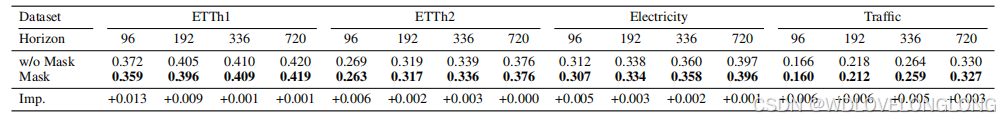
表 3:在 ETT 数据集上使用 MMFNet 进行多变量 LTSF 的 MSE 结果(带或不带掩蔽模块)。“Mask” 表示带掩蔽模块的结果,而“w/o Mask” 表示不带掩蔽模块的结果。“Imp.”表示掩蔽模块带来的改进。
To evaluate the effectiveness of the self-adaptive masking mechanism, we compare MMFNet’s performance on the ETT dataset with and without the masking module across four forecast horizons: 96,
192
,
336
, and
720
. As Table 3 lists, MMFNet with masking consistently outperforms the version without masking across all horizons. The most notable improvements occur at the horizon 96
with a 3
.
5%
MSE reduction on ETTh1 (+0.013) and a
2
.
2%
MSE reduction on ETTh2 (+0.006). With the Electricity dataset, the largest improvement is at horizon 96
with an improvement of
+0
.
005
. Similarly, the largest improvement is at horizon 192
with an improvement of
+0
.
006
on the Traffic dataset. The results show that the self-adaptive masking mechanism which filters out frequency noise at different scales consistently enhances forecasting accuracy across various datasets and forecast horizons. A more detailed analysis of the mask output is provided in Appendix C
为了评估自适应掩蔽机制的有效性,我们在四个预测时限(96、192、336 和 720)上比较了 MMFNet 在 ETT 数据集上使用和不使用掩蔽模块的性能。如表 3 所列,在所有时限上,带掩蔽的 MMFNet 始终优于不带掩蔽的版本。最显著的改进发生在时限 96,ETTh1 的 MSE 降低了 3.5%(+0.013),ETTh2 的 MSE 降低了 2.2%(+0.006)。对于电力数据集,最大的改进是在时限 96,改进了 +0.005。同样,最大的改进是在时限 192,交通数据集的改进了 +0.006。结果表明,自适应掩蔽机制可以滤除不同尺度的频率噪声,从而持续提高各种数据集和预测时限的预测准确性。附录 C 中提供了有关掩码输出的更详细分析。
4.5 P
ERFORMANCE ON
U
LTRA
-
LONG
-
TERM
T
IME
S
ERIES
F
ORECASTING
Table 4: MSE results for multivariate ultra long-term time series forecasting with MMFNet. The
best result is emphasized in
bold
, while the second-best is underlined. “Imp.” represents the im
provement between MMFNet and either the best or second-best result, with a higher “Imp.” value
indicating greater improvement.
4.5 超长期时间序列预测性能
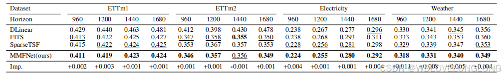
表 4:使用 MMFNet 进行多变量超长期时间序列预测的 MSE 结果。
最佳结果以粗体突出显示,而第二佳结果则用下划线表示。“Imp.”表示 MMFNet 与最佳或第二佳结果之间的改进,“Imp.”值越高,表示改进越大。
We evaluate MMFNet’s performance in ultra-long-term time series forecasting scenarios. Table 4
presents the MSE results for various models applied to multivariate ultra-long-term time series forecasting across four datasets at forecast horizons of 960, 1200, 1440, and 1680. Due to the significantmemory requirements of models such as FEDformer, TimesNet, TimeMixer, and PatchTST whenforecast horizons are extended, these models exceed GPU memory limitations. Consequently, in this context, we limit the comparison to more lightweight models: DLinear, FITS, SparseTSF, and the proposed MMFNet.
我们评估了 MMFNet 在超长期时间序列预测场景中的表现。表 4 展示了在四个数据集中应用于多元超长期时间序列预测的各种模型的 MSE 结果,预测范围分别为 960、1200、1440 和 1680。由于 FEDformer、TimesNet、TimeMixer 和 PatchTST 等模型在扩展预测范围时对内存的需求很大,这些模型超出了 GPU 内存限制。因此,在这种情况下,我们将比较限制在更轻量级的模型上:DLinear、FITS、SparseTSF 和提出的 MMFNet。
The results show that MMFNet consistently outperforms the existing models across most datasets and forecast horizons. For example, with the ETTh1 dataset, MMFNet achieves the MSE values of 0.411, 0.419, 0.423, and 0.424 at horizons of 960, 1200, 1440, and 1680, respectively. With the Electricity dataset, MMFNet delivers very good performance, particularly at longer horizons, with the MSE values of 0.255 at 1200 and 0.292 at 1680.On the Weather dataset, MMFNet demonstrates superior performance, achieving MSE values of 0.318 at the 960 horizon and 0.331 at the 1200 horizon, representing a 3.3% (+0.011) and 2.4% (+0.008) reduction in MSE compared to the second-best baseline. The results demonstrate the robustness of MMFNet in forecasting multivariate ultra-long-term time series data across various datasets and extended forecast horizons by effectively capturing frequency variations at different scales.
结果表明,MMFNet 在大多数数据集和预测期内始终优于现有模型。例如,对于 ETTh1 数据集,MMFNet 在 960、1200、1440 和 1680 的预测期内分别实现了 0.411、0.419、0.423 和 0.424 的 MSE 值。对于电力数据集,MMFNet 提供了非常好的性能,特别是在较长的预测期内,1200 时的 MSE 值为 0.255,1680 时的 MSE 值为 0.292。在天气数据集上,MMFNet 表现出色,在 960 的预测期内实现了 0.318 的 MSE 值,在 1200 的预测期内实现了 0.331 的 MSE 值,与第二好的基线相比,MSE 分别降低了 3.3% (+0.011) 和 2.4% (+0.008)。结果表明,MMFNet 通过有效捕捉不同尺度的频率变化,在预测各种数据集和扩展预测范围内的多元超长期时间序列数据方面具有很强的稳健性。
5 R
ELATED
W
ORK
5.1 L
ONG
-
TERM
T
IME
S
ERIES
F
ORECASTING
LTSF is a critical area in data science and machine learning and focuses on predicting future values over extended periods. Such a task is challenging due to the inherent seasonality, trends, and noise in time series data. In addition, time series data is often complex and high-dimensional Zheng et al. (2024; 2023). Traditional statistical methods, such as ARIMA (Contreras et al., 2003) and Holt-Winters (Chatfield & Yar, 1988), are effective for short-term forecasting but frequently fall
short for longer horizons. Machine learning models, such as SVM (Wang & Hu, 2005), Random
Forests Breiman (2001), and Gradient Boosting Machines (Natekin & Knoll, 2013), offer improved
performance by capturing non-linear relationships but typically require extensive feature engineering. Recently, deep learning models, such as RNNs, LSTMs, GRUs, and Transformer-based models (Informer and Autoformer), have demonstrated notable efficiency in modeling long-term dependencies. Furthermore, the hybrid models that combine statistical methods with machine learning or deep learning techniques have shown improved accuracy. State-of-the-art models, such as FEDformer (Zhou et al., 2022b), FiLM (Zhou et al., 2022a), PatchTST Nie et al. (2024), and SparseTSF, leverage frequency domain transformations and efficient self-attention to improve prediction performance.
5 相关工作
5.1 长期时间序列预测
LTSF 是数据科学和机器学习中的一个重要领域,专注于预测长期的未来值。由于时间序列数据固有的季节性、趋势和噪声,这样的任务具有挑战性。此外,时间序列数据通常很复杂且维度很高(Zheng 等人,2024;2023)。传统统计方法,如 ARIMA(Contreras 等人,2003)和 Holt-Winters(Chatfield & Yar,1988),对于短期预测有效,但对于较长的预测范围往往不够。机器学习模型,如 SVM(Wang & Hu,2005)、随机森林 Breiman(2001)和梯度提升机(Natekin & Knoll,2013),通过捕捉非线性关系提供了改进的性能,但通常需要大量的特征工程。最近,深度学习模型(例如 RNN、LSTM、GRU 和基于 Transformer 的模型(Informer 和 Autoformer))在长期依赖关系建模方面表现出了显著的效率。此外,将统计方法与机器学习或深度学习技术相结合的混合模型也表现出了更高的准确性。最先进的模型(例如 FEDformer(Zhou 等人,2022b)、FiLM(Zhou 等人,2022a)、PatchTST Nie 等人(2024)和 SparseTSF)利用频域变换和高效的自注意力来提高预测性能。
5.2 T
IME
S
ERIES
F
ORECASTING IN THE
F
REQUENCY
D
OMAIN
Recent advancements in time series analysis have increasingly utilized frequency domain information to reveal underlying patterns. For instance, FNet (Lee-Thorp et al., 2021) adopts an attention based approach to capture temporal dependencies within the frequency domain, thereby eliminating the need for convolutional or recurrent layers. Models such as FEDformer (Zhou et al., 2022b) and FiLM (Zhou et al., 2022a) improve predictive performance by incorporating frequency domain information as auxiliary features. FITS (Xu et al., 2024) also demonstrates strong predictive capabilities by converting time-domain forecasting tasks into the frequency domain and utilizing low-pass filters to reduce the number of parameters required. However, many of these techniques rely on manual feature engineering to identify dominant periods, which can constrain the amount of information captured and introduce inefficiencies or risks of overfitting.
5.2 频域中的时间序列预测
时间序列分析的最新进展越来越多地利用频域信息来揭示潜在的模式。例如,FNet(Lee-Thorp 等人,2021 年)采用基于注意力的方法来捕获频域内的时间依赖性,从而无需卷积层或循环层。FEDformer(Zhou 等人,2022b)和 FiLM(Zhou 等人,2022a)等模型通过将频域信息作为辅助特征来提高预测性能。FITS(Xu 等人,2024 年)还通过将时域预测任务转换为频域并利用低通滤波器减少所需参数的数量来展示强大的预测能力。然而,这些技术中的许多都依赖于手动特征工程来识别主要周期,这可能会限制捕获的信息量并导致效率低下或过度拟合的风险。
5.3 M
ULTISCALING
M
ODEL
In the field of computer vision, several multi-scale Vision Transformers (ViTs) have leveraged hi
erarchical architectures to generate progressively down-sampled pyramid features. For instance,
Multi-Scale Vision Transformers (Fan et al., 2021) enhance the standard Vision Transformer architecture by incorporating multi-scale processing, allowing for improved detail capture across varying spatial resolutions. Pyramid Vision Transformer (Wang et al., 2021) integrates a pyramid structure within ViTs to facilitate multi-scale feature extraction, while Twins (Dai et al., 2021) combines local and global attention to effectively model multi-scale representations. SegFormer (Xieet al., 2021) introduces an efficient hierarchical encoder that captures both coarse and fine features, and CSWin (Dong et al., 2022) further improves performance by using multi-scale cross-shaped local attention mechanisms. In the context of time series forecasting, TimeMixer (Wang et al., 2024) represents a significant advancement with its fully MLP-based architecture, which employs Past-Decomposable-Mixing and Future-Multipredictor-Mixing blocks. This architecture enables TimeMixer to effectively leverage disentangled multi-scale time series data during both past extraction and future prediction phases.
5.3 多尺度模型
在计算机视觉领域,多个多尺度视觉变换器 (ViT) 利用分层架构来生成逐步下采样的金字塔特征。例如,多尺度视觉变换器 (Fan 等人,2021) 通过结合多尺度处理增强了标准视觉变换器架构,从而可以在不同的空间分辨率下更好地捕获细节。金字塔视觉变换器 (Wang 等人,2021) 在 ViT 中集成了金字塔结构以促进多尺度特征提取,而 Twins (Dai 等人,2021) 结合了局部和全局注意力来有效地模拟多尺度表示。 SegFormer (Xieet al., 2021) 引入了一种高效的分层编码器,可以捕获粗略和精细特征,而 CSWin (Dong et al., 2022) 通过使用多尺度十字形局部注意机制进一步提高了性能。在时间序列预测的背景下,TimeMixer (Wang et al., 2024) 凭借其完全基于 MLP 的架构取得了重大进步,该架构采用了过去可分解混合和未来多预测器混合块。这种架构使 TimeMixer 能够在过去提取和未来预测阶段有效利用解缠结的多尺度时间序列数据。
5.4 M
ASKED
M
ODELING
Masked language modeling and its autoregressive variants have emerged as dominant self
supervised learning approaches in natural language processing. These techniques enable large-scale language models to excel in both language understanding and generation by predicting masked or hidden tokens within sentences (Devlin et al., 2018; Radford et al., 2018). In computer vision, early approaches, such as the context encoder (Pathak et al., 2016), involve masking specific regions of an image and predicting the missing pixels, while Contrastive Predictive Coding (van den Oord et al., 2018) uses contrastive learning to improve feature representations. Recent innovations in MIM include models like iGPT (Chen et al., 2020), ViT (Dosovitskiy et al., 2021), and BEiT (Bao et al., 2022), which leverage Vision Transformers and techniques, such as pixel clustering, mean color prediction, and block-wise masking. In the realm of multivariate time series forecasting, masked encoders have recently been employed with notable success in classification and regression tasks (Zerveas et al., 2021). For example, PatchTST uses a masked self-supervised representation learning method to reconstruct the masked patches and showcases its effectiveness in time series data (Nie et al., 2024). However, the application of masked modeling techniques in linear time series forecasting remains relatively under-explored.
5.4 掩蔽建模
掩蔽语言建模及其自回归变体已成为自然语言处理中占主导地位的自监督学习方法。这些技术通过预测句子中的掩蔽或隐藏标记,使大规模语言模型在语言理解和生成方面表现出色(Devlin 等人,2018 年;Radford 等人,2018 年)。在计算机视觉中,早期的方法(例如上下文编码器(Pathak 等人,2016 年))涉及掩蔽图像的特定区域并预测缺失的像素,而对比预测编码(van den Oord 等人,2018 年)使用对比学习来改进特征表示。 MIM 的最新创新包括 iGPT(Chen 等人,2020 年)、ViT(Dosovitskiy 等人,2021 年)和 BEiT(Bao 等人,2022 年)等模型,它们利用了 Vision Transformers 和像素聚类、平均颜色预测和逐块掩码等技术。在多元时间序列预测领域,掩码编码器最近已在分类和回归任务中取得了显著的成功(Zerveas 等人,2021 年)。例如,PatchTST 使用掩码自监督表示学习方法来重建掩码补丁,并展示了其在时间序列数据中的有效性(Nie 等人,2024 年)。然而,掩码建模技术在线性时间序列预测中的应用仍然相对未被充分探索。
6 C
ONCLUSION
MMFNet significantly advances long-term multivariate forecasting by employing the MMFT approach. Through comprehensive evaluations on benchmark datasets, we have demonstrated that MMFNet consistently outperforms state-of-the-art models in forecasting accuracy, highlighting its robustness in capturing complex data patterns. By effectively integrating multi-scale decomposition with a learnable masked filter, MMFNet captures intricate temporal details while adaptively mitigating noise, making it a versatile and reliable solution for a wide range of LTSF tasks.
6 结论
MMFNet 通过采用 MMFT 方法显著推进了长期多元预测。通过对基准数据集的全面评估,我们证明了 MMFNet 在预测准确性方面始终优于最先进的模型,凸显了其在捕获复杂数据模式方面的稳健性。通过有效地将多尺度分解与可学习的掩蔽滤波器相结合,MMFNet 可以捕获复杂的时间细节,同时自适应地减轻噪声,使其成为适用于各种 LTSF 任务的多功能可靠解决方案。
三、SCALEFORMER:用于时间序列预测的迭代多尺度细化变换器
The performance of time series forecasting has recently been greatly improved by the introduction of transformers. In this paper, we propose a general multi-scale framework that can be applied to the state-of-the-art transformer-based time series forecasting models (FEDformer, Autoformer, etc.). By iteratively refining a forecasted time series at multiple scales with shared weights, introducing architecture adaptations, and a specially-designed normalization scheme, we are able to achieve significant performance improvements, from 5
.
5%
to
38
.
5%
across datasets and transformer architectures, with minimal additional computational overhead. Via
detailed ablation studies, we demonstrate the effectiveness of each of our contributions across the architecture and methodology. Furthermore, our experiments on various public datasets demonstrate that the proposed improvements outperform their corresponding baseline counterparts. Our code is publicly available in
https://github.com/BorealisAI/scaleformer
.
最近,由于引入了 Transformer,时间序列预测的性能得到了极大改善。在本文中,我们提出了一个通用的多尺度框架,该框架可应用于最先进的基于 Transformer 的时间序列预测模型(FEDformer、Autoformer 等)。通过使用共享权重在多个尺度上迭代细化预测的时间序列、引入架构适配和专门设计的规范化方案,我们能够实现显着的性能改进,从 5.5% 到 38.5% 的跨数据集和 Transformer 架构,同时将额外的计算开销降至最低。通过详细的消融研究,我们展示了我们每一项贡献在架构和方法上的有效性。此外,我们在各种公共数据集上的实验表明,所提出的改进优于其相应的基线对应物。我们的代码可在 https://github.com/BorealisAI/scaleformer 上公开获取。
Integrating information at different time scales is essential to accurately model and forecast time series (
Mozer
,
1991
;
Ferreira et al.
,
2006
). From weather patterns that fluctuate both locally and globally, as well as throughout the day and across seasons and years, to radio carrier waves which contain relevant signals at different frequencies, time series forecasting models need to encourage scale awareness
in learnt representations. While transformer-based architectures have become the mainstream and stateof-the-art for time series forecasting in recent years,
advances have focused mainly on mitigating the standard quadratic complexity in time and space, e.g., attention (
Li et al.
,
2019
;
Zhou et al.
,
2021
) or structural changes (
Xu et al.
,
2021
;
Zhou et al.
,
2022b
), rather than explicit scale-awareness. The essential cross-scale feature relationships are often learnt implicitly, and are not encouraged by architectural priors of any kind beyond the stacked attention blocks that characterize the transformer models. Autoformer (
Xu
et al.
,
2021
) and Fedformer (
Zhou et al.
,
2022b
) introduced some emphasis on scale-awareness by enforcing different computational paths for the trend and seasonal components of the input time series; however, this structural prior only focused on two scales: low- and high-frequency components.
Given their importance to forecasting, can we make transformers more scale-aware?
整合不同时间尺度的信息对于准确建模和预测时间序列至关重要(Mozer,1991;Ferreira 等人,2006)。从在本地和全球范围内以及全天、跨季节和跨年份波动的天气模式,到包含不同频率相关信号的无线电载波,时间序列预测模型需要在学习的表示中鼓励尺度意识。虽然基Transformer 的架构近年来已成为时间序列预测的主流和最先进技术,但进展主要集中在减轻时间和空间的标准二次复杂度上,例如注意力(Li 等人,2019;Zhou 等人,2021)或结构变化(Xu 等人,2021;Zhou 等人,2022b),而不是明确的尺度意识。基本的跨尺度特征关系通常是隐式学习的,除了表征 Transformer 模型的堆叠注意力块之外,任何类型的架构先验都不会鼓励这种关系。Autoformer(Xu 等人,2021 年)和 Fedformer(Zhou 等人,2022b 年)通过对输入时间序列的趋势和季节性成分实施不同的计算路径,引入了一些对尺度感知的强调;然而,这种结构先验只关注两个尺度:低频和高频成分。鉴于它们对预测的重要性,我们能否让 Transformer 更具尺度感知能力
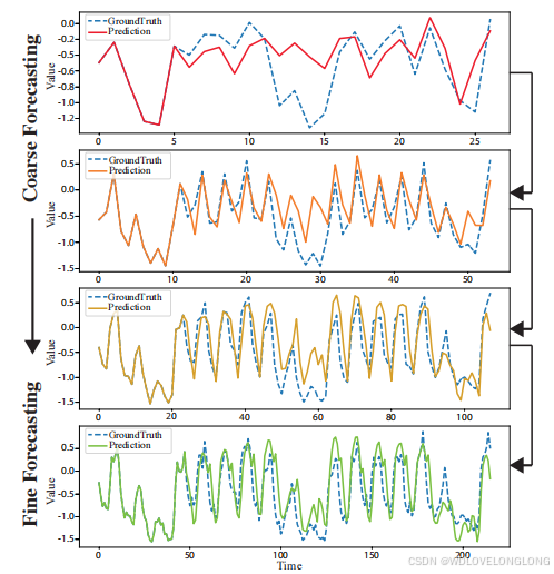
Figure 1: Intermediate forecasts by our model at different time scales. Iterative refinement
of a time series forecast is a strong structural prior that benefits time series forecasting.
图 1:我们的模型在不同时间尺度上的中期预测。时间序列预测的迭代细化是一种强大的结构先验,有利于时间序列预测。
We enable this scale-awareness with
Scaleformer
. In our proposed approach, showcased in Figure
1
, time series forecasts are iteratively refined at successive time-steps, allowing the model to better capture the inter-dependencies and specificities of each scale. However, scale itself is not sufficient. Iterative refinement at different scales can cause significant distribution shifts between intermediate forecasts which can lead to runaway error propagation. To mitigate this issue, we introduce cross-scale normalization at each step.
我们利用 Scaleformer 实现了这种尺度感知。在我们提出的方法中(如图 1 所示),时间序列预测在连续的时间步骤中迭代细化,从而使模型能够更好地捕捉每个尺度的相互依赖性和特异性。然而,尺度本身是不够的。不同尺度的迭代细化可能会导致中间预测之间的分布发生显著变化,从而导致失控误差传播。为了缓解这个问题,我们在每个步骤中引入了跨尺度标准化。
Our approach re-orders model capacity to shift the focus on scale awareness, but does not fundamentally alter the attention-driven paradigm of transformers. As a result, it can be readily adapted to work jointly with multiple recent time series transformer architectures, acting broadly orthogonally to their own contributions. Leveraging this, we chose to operate with various transformer-based backbones (e.g. Fedformer, Autoformer, Informer, Reformer, Performer) to further probe the effect of our multi-scale method on a variety of experimental setups.
我们的方法重新排序了模型容量,将重点转移到尺度感知上,但并没有从根本上改变 Transformer 的注意力驱动范式。因此,它可以很容易地与多个最近的时间序列 Transformer 架构协同工作,与它们自己的贡献大致正交。利用这一点,我们选择使用各种基于 Transformer 的主干(例如 Fedformer、Autoformer、Informer、Reformer、Performer),以进一步探究我们的多尺度方法对各种实验设置的影响。
Our contributions are as follows: (1) we introduce a novel iterative scale-refinement paradigm that
can be readily adapted to a variety of transformer-based time series forecasting architectures. (2) To minimize distribution shifts between scales and windows, we introduce cross-scale normalization on outputs of the Transformer. (3) Using Informer and AutoFormer, two state-of-the-art architectures, as backbones, we demonstrate empirically the effectiveness of our approach on a variety of datasets. Depending on the choice of transformer architecture, our mutli-scale framework results in mean squared error reductions ranging from 5
.
5%
to
38
.
5%
. (4) Via a detailed ablation study of our findings, we demonstrate the validity of our architectural and methodological choices.
我们的贡献如下:(1)我们引入了一种新颖的迭代尺度细化范式,
该范式可以轻松适应各种基于 Transformer 的时间序列预测架构。(2)为了最大限度地减少尺度和窗口之间的分布偏移,我们在 Transformer 的输出上引入了跨尺度规范化。(3)使用 Informer 和 AutoFormer(两种最先进的架构)作为主干,我们通过经验证明了我们的方法在各种数据集上的有效性。根据 Transformer 架构的选择,我们的多尺度框架可将均方误差降低 5.5% 到 38.5%。(4)通过对我们的研究结果进行详细的消融研究,我们证明了我们的架构和方法选择的有效性。
2 R
ELATED WORKS
Time-series forecasting
: Time-series forecasting plays an important role in many domains, including: weather forecasting (
Murphy
,
1993
), inventory planning (
Syntetos et al.
,
2009
), astronomy (
Scargle
,
1981
), economic and financial forecasting (
Krollner et al.
,
2010
). One of the specificities of time series data is the need to capture seasonal
trends (
Brockwell & Davis
,
2009
). There exits a vast variety of time-series forecasting models (
Box & Jenkins
,
1968
;
Hyndman et al.
,
2008
;
Salinas et al.
,
2020
;
Rangapuram et al.
,
2018
;
Bai et al.
,
2018
;
Wu et al.
,
2020
). Early approaches such as ARIMA (
Box & Jenkins
,
1968
) and exponential smoothing models (
Hyndman et al.
,
2008
) were followed by the introduction of neural network based approaches involving either Recurrent Neural Netowkrs (RNNs) and their variants (
Salinas et al.
,
2020
;
Rangapuram et al.
,
2018
;
Salinas et al.
,
2020
) or Temporal Convolutional Networks (TCNs) (
Bai et al.
,
2018
).
More recently, time-series Transformers (
Wu et al.
,
2020
;
Zerveas et al.
,
2021
;
Tang & Matteson
,
2021
) were introduced for the forecasting task by leveraging self-attention mechanisms to learn
complex patterns and dynamics from time series data. Informer (
Zhou et al.
,
2021
) reduced quadratic complexity in time and memory to O
(
L
log
L
)
by enforcing sparsity in the attention mechanism with the ProbSparse attention. Yformer (
Madhusudhanan et al.
,
2021
) proposed a Y-shaped encoderdecoder architecture to take advantage of the multi-resolution embeddings. Autoformer (
Xu et al.
,
2021
) used a cross-correlation-based attention mechanism to operate at the level of subsequences. FEDformer (
Zhou et al.
,
2022b
) employs frequency transform to decompose the sequence into multiple frequency domain modes to extract the feature, further improving the performance of Autoformer.
2 相关作品
时间序列预测:时间序列预测在许多领域发挥着重要作用,包括:天气预报(Murphy,1993 年)、库存规划(Syntetos 等,2009 年)、天文学(Scargle,1981 年)、经济和金融预测(Krollner 等,2010 年)。时间序列数据的一个特性是需要捕捉季节性趋势(Brockwell & Davis,2009 年)。存在各种各样的时间序列预测模型(Box & Jenkins,1968 年;Hyndman 等,2008 年;Salinas 等,2020 年;Rangapuram 等,2018 年;Bai 等,2018 年;Wu 等,2020 年)。早期的方法,例如 ARIMA(Box & Jenkins,1968)和指数平滑模型(Hyndman 等人,2008),随后引入了基于神经网络的方法,包括循环神经网络 (RNN) 及其变体(Salinas 等人,2020;Rangapuram 等人,2018;Salinas 等人,2020)或时间卷积网络 (TCN)(Bai 等人,2018)。最近,时间序列 Transformer(Wu 等人,2020;Zerveas 等人,2021;Tang & Matteson,2021)被引入用于预测任务,通过利用自注意力机制从时间序列数据中学习复杂的模式和动态。 Informer (Zhou et al., 2021) 通过使用 ProbSparse 注意力机制强制稀疏性,将时间和内存的二次复杂度降低到 O(Llog L)。Yformer (Madhusudhanan et al., 2021) 提出了一种 Y 形编码器解码器架构,以利用多分辨率嵌入。Autoformer (Xu et al., 2021) 使用基于互相关的注意力机制在子序列级别进行操作。FEDformer (Zhou et al., 2022b) 使用频率变换将序列分解为多个频域模式以提取特征,进一步提高了 Autoformer 的性能。
Multi-scale neural architectures
: Multi-scale and hierarchical processing is useful in many domains, such as computer vision (
Fan et al.
,
2021
;
Zhang et al.
,
2021
;
Liu et al.
,
2018
), natural language processing (
Nawrot et al.
,
2021
;
Subramanian et al.
,
2020
;
Zhao et al.
,
2021
) and time series forecasting (
Chen et al.
,
2022
;
Ding et al.
,
2020
). Multiscale Vision Transformers (
Fan et al.
,
2021
) is proposed for video and image recognition, by connecting the seminal idea of multiscale feature hierarchies with transformer models, however, it focuses on the spatial domain, specially designed for computer vision tasks.
Cui et al.
(
2016
) proposed to use different transformations of a time series such as downsampling and smoothing in parallel to the original signal to better capture temporal patterns and reduce the effect of random noise. Many different architectures have been proposed recently (
Chung et al.
,
2016
;
Che et al.
,
2018
;
Shen et al.
,
2020
;
Chen et al.
,
2021
) to improve RNNs in tasks such as language processing, computer vision, time-series analysis, and speech recognition. However, these methods are mainly focused on proposing a new RNN-based module which is not applicable to transformers directly. The same direction has been also investigated in Transformers, TCN, and MLP models. Recent work
Du et al.
(
2022
) proposed multi-scale segment-wise correlations as a multi-scale version of the self-attention mechanism. Our work is orthogonal to the above methods as a model-agnostic framework to utilize multi-scale time-series in transformers while keeping the
number of parameters and time complexity roughly the same.
多尺度神经架构:多尺度和分层处理在许多领域都很有用,例如计算机视觉(Fan 等人,2021 年;Zhang 等人,2021 年;Liu 等人,2018 年)、自然语言处理(Nawrot 等人,2021 年;Subramanian 等人,2020 年;Zhao 等人,2021 年)和时间序列预测(Chen 等人,2022 年;Ding 等人,2020 年)。多尺度视觉变换器(Fan 等人,2021 年)是为视频和图像识别而提出的,它将多尺度特征层次的开创性思想与变换器模型相结合,但它专注于空间域,专为计算机视觉任务而设计。崔等人。 (2016)建议对时间序列使用不同的变换,例如与原始信号并行的下采样和平滑,以更好地捕获时间模式并减少随机噪声的影响。最近提出了许多不同的架构(Chung 等人,2016;Che 等人,2018;Shen 等人,2020;Chen 等人,2021)来改进 RNN 在语言处理、计算机视觉、时间序列分析和语音识别等任务中的表现。然而,这些方法主要集中在提出一种新的基于 RNN 的模块,它不直接适用于 Transformer。Transformer、TCN 和 MLP 模型中也研究了同样的方向。最近的研究 Du 等人(2022)提出了多尺度分段相关性作为自注意力机制的多尺度版本。我们的工作与上述方法正交,作为一个与模型无关的框架,在 Transformer 中利用多尺度时间序列,同时保持参数数量和时间复杂度大致相同。
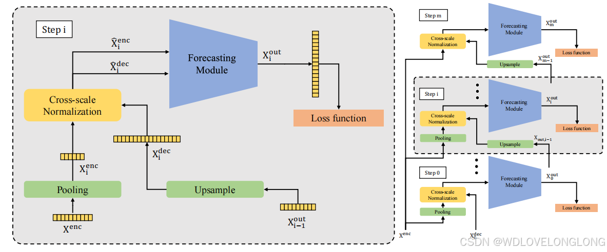
Figure 2: Overview of the proposed
Scaleformer
framework. (Left) Representation of a single scale block. In each step, we pass the normalized upsampled output from previous step along with the normalized downsampled encoder as the input. (Right) Representation of the full architecture. We process the input in a multi-scale manner iteratively from the smallest scale to the original scale.
图 2:所提出的 Scaleformer 框架的概览。(左)单个尺度块的表示。在每个步骤中,我们将上一步的归一化上采样输出与归一化下采样编码器一起作为输入传递。(右)完整架构的表示。我们以多尺度方式迭代处理输入,从最小尺度到原始尺度。
3 M
ETHOD
In this section, we first introduce the problem setting in Sec.
3.1
, then describe the proposed
framework in Sec.
3.2
, and the normalization scheme in Sec.
3.3
. We provide details on the input’s representation in Sec.
3.4
, and the loss function in Sec.
3.5
.
3 方法
在本节中,我们首先在第 3.1 节中介绍问题设置,然后在第 3.2 节中描述所提出的框架,并在第 3.3 节中描述规范化方案。我们在第 3.4 节中详细介绍了输入的表示,并在第 3.5 节中详细介绍了损失函数。
3.1 P
ROBLEM
S
ETTING
We denote
X
(
L
)
and
X
(
H
)
the look-back and horizon windows for the forecast, respectively, of
corresponding lengths
`
L
, `
H
. Given a starting time
t
0
we can express these time-series of dimension
d
x
, as follows:
X
(
L
)
=
{
x
t
|
x
t
∈
R
d
x
, t
∈
[
t
0
, t
0
+
`
L
]
}
and
X
(
H
)
=
{
x
t
|
x
t
∈
R
d
x
, t
∈
[
t
0
+
`
L
+ 1, t
0
+
`
L
+
`
H
]
}
. The goal of the forecasting task is to predict the horizon window
X
(
H
)
given the look-back window X
(
L
)
.
3.1 问题设置
我们分别用 X(L) 和 X(H) 表示预测的回顾窗口和展望窗口,相应的长度为 ` L, ` H。给定起始时间 t0,我们可以将这些维度为 dx 的时间序列表示如下:X(L) = {xt|xt ∈ R dx , t ∈ [t0, t0 + ` L]} 和 X(H) = {xt|xt ∈ R dx , t ∈ [t0 + ` L + 1, t0 + ` L + ` H]}。预测任务的目标是根据回顾窗口 X(L) 预测展望窗口 X(H)。
3.2 M
ULTI
-
SCALE
F
RAMEWORK
Our proposed framework applies successive transformer modules to iteratively refine a time-series forecast, at different temporal scales. The proposed framework is shown in Figure
2
.
Given an input time-series
X
(
L
)
, we iteratively apply the same neural module mutliple times at
different temporal scales. Concretely, we consider a set of scales
S
=
{
s
m
, ..., s
2
, s
1
,
1
}
(i.e. for the default scale of s
= 2
,
S
is a set of consecutive powers of
2
), where
m
=
b
log
s
`
L
c −
1
and
s
is a downscaling factor. The input to the encoder at the i
-th step (
0
≤
i
≤
m
) is the original look-back window X
(
L
)
, downsampled by a scale factor of
s
i
≡
s
m
−
i
via an average pooling operation. The input to the decoder, on the other hand, is X
out
i
−
1
upsampled by a factor of
s
via a linear interpolation.
Finally,
X
dec
0
is initialized to an array of 0s. The model performs the following operations:
3.2 多尺度框架
我们提出的框架应用连续的变换器模块在不同的时间尺度上迭代细化时间序列预测。所提出的框架如图 2 所示。给定一个输入时间序列 X(L) ,我们在不同的时间尺度上迭代多次应用相同的神经模块。具体来说,我们考虑一组尺度 S = {s m, ..., s2 , s1 , 1}(即对于默认尺度 s = 2,S 是一组连续的 2 的幂),其中 m = b log ` Lc − 1 ,s 是降尺度因子。第 i 步(0 ≤ i ≤ m)编码器的输入是原始回溯窗口 X(L) ,通过平均池化操作以 si ≡ s m−i 的比例因子进行降采样。另一方面,解码器的输入是 Xout i−1,通过线性插值以 s 倍上采样。最后,Xdec 0 被初始化为 0 的数组。该模型执行以下操作:
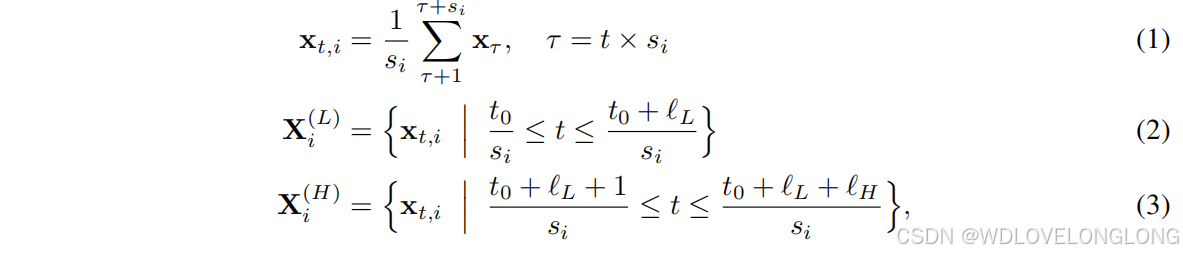
where
X
(
i L
)
and
X
(
i H
)
are the look-back and horizon windows at the
i
th step at time t with the scale factor of s
m
−
i
and with the lengths of
`
L,i
and
`
H,i
, respectively. Assuming
x
0
t,i
−
1
is the output of the forecasting module at step i
−
1
and time
t
, we can define
X
enc
i
and
X
dec
i
as the inputs to the normalization:
其中 X ( i L) 和 X ( i H) 分别是时间 t 时第 i 步的回顾窗口和水平窗口,比例因子为 s m−i,长度分别为 ` L,i 和 ` H,i。假设 x 0 t,i−1 是步骤 i − 1 和时间 t 的预测模块的输出,我们可以将 Xenc i 和 Xdec i 定义为归一化的输入:
Finally, we calculate the error between
X
(
i H
)
and
X
out
i
as the loss function to train the model. Please refer to Algorithm
1
for details on the sequence of operations performed during the forward pass.
最后,我们计算 X ( i H) 和 Xout i 之间的误差作为损失函数来训练模型。有关前向传递过程中执行的操作序列的详细信息,请参阅算法 1。
3.3 C
ROSS
-
SCALE
N
ORMALIZATION
Given a set of input series (
X
enc
i
,
X
dec
i
), with dimensions
`
L
i
×
d
x
and
`
H
i
×
d
x
, respectively for the encoder and the decoder of the transformer in i
th step, we normalize each series based on the temporal average of X
enc
i
and
X
dec
i
. More formally:
3.3 跨尺度归一化
给定一组输入序列 (Xenc i , Xdec i ),其维度分别为 ` Li × dx 和 ` Hi × dx,分别用于第 i 步 Transformer 的编码器和解码器,我们基于 Xenc i 和 Xdec i 的时间平均值对每个序列进行归一化。更正式地:
where
µ
¯
X
i
∈
R
d
x
is the average over the temporal dimension of the concatenation of both look-back window and the horizon. Here, X
ˆ
enc
i
and
X
ˆ
dec
i
are the inputs of the
i
th step to the forecasting module.
其中 µ¯Xi ∈ R dx 是回顾窗口和范围的串联在时间维度上的平均值。这里,Xˆ enc i 和 Xˆ dec i 是第 i 步对预测模块的输入。
Figure 3: The figure shows the output results of two series using the same trained multi-scale model with and without shifting the data (left) which demonstrates the importance of normalization. On the right, we can see the distribution changes due to the downsampling of two series compared to the original scales from the Electricity dataset.
图 3:该图显示了使用相同训练过的多尺度模型对两个序列进行移位和不移位时的输出结果(左),这说明了规范化的重要性。在右侧,我们可以看到由于两个序列的下采样导致的分布变化,与电力数据集的原始尺度相比。
Distribution shift is when the distribution of input to a model or its sub-components changes across training to deployment (
Shimodaira
,
2000
;
Ioffe & Szegedy
,
2015
). In our context, two distinct distribution shifts are common. First, there is a natural distribution shift between the look-back and the forecast window (the covariate shift). Additionally, there is a distribution shift
between the predicted forecast windows at two consecutive scales which is a result of the upsampling operation alongside the error accumulation during the intermediate computations. As a result, normalizing the output at a given step by either the look-back window statistics or the previously predicted forecast window statistics result in an accumulation of errors across steps. We mitigate this by considering a moving average of forecast and look-back statistics as the basis for the output normalization. While this change might appear relatively minor, it has a significant impact on the resulting distribution of outputs. The improvement is more evident when compared to the alternative approaches, namely, normalizing by either look-back or previous forecast window statistics.
分布偏移是指模型或其子组件的输入分布在训练和部署过程中发生变化(Shimodaira,2000;Ioffe & Szegedy,2015)。在我们的上下文中,两种不同的分布偏移很常见。首先,回顾窗口和预测窗口之间存在自然的分布偏移(协变量偏移)。此外,两个连续尺度的预测预测窗口之间存在分布偏移 ,这是上采样操作以及中间计算过程中的误差累积的结果。因此,通过回顾窗口统计数据或先前预测的预测窗口统计数据对给定步骤的输出进行归一化会导致步骤间误差的累积。我们通过将预测和回顾统计数据的移动平均值视为输出归一化的基础来缓解这种情况。虽然这种变化可能看起来相对较小,但它对最终的输出分布有重大影响。与其他方法(即通过回顾或先前的预测窗口统计数据进行归一化)相比,这种改进更为明显。
3.4 I
NPUT
E
MBEDDING
Following the previous works, we embed our input to have the same number of features as the hidden dimension of the model. The embedding consists of three parts: (1) Value embedding
which uses a linear layer to map the input observations of each step x
t
to the same dimension as the model. We further concatenate an additional value 0
,
0
.
5
, or
1
respectively showing if each observation is coming from the look-back window, zero initialization, or the prediction of the previous steps. (2) Temporal
Embedding
which again uses a linear layer to embed the time stamp related to each observation to the hidden dimension of the model. Here we concatenate an additional value 1
/s
i
−
0
.
5
as the current scale for the network before passing to the linear layer. (3) We also use a fixed positional embedding which is adapted to the different scales s
i
as follows:
3.4 输入嵌入
根据之前的研究,我们将输入嵌入为具有与模型隐藏维度相同数量的特征。嵌入由三部分组成:(1)值嵌入,使用线性层将每个步骤 xt 的输入观察映射到与模型相同的维度。我们进一步连接一个附加值 0、0.5 或 1,分别显示每个观察是来自回顾窗口、零初始化还是前几步的预测。(2)时间嵌入,再次使用线性层将与每个观察相关的时间戳嵌入到模型的隐藏维度。在这里,我们在传递到线性层之前连接一个附加值 1/si − 0.5 作为网络的当前尺度。(3)我们还使用固定位置嵌入,该嵌入适用于不同的尺度 si,如下所示:

3.5 L
OSS
F
UNCTION
Using the standard MSE objective to train time-series forecasting models leaves them sensitive
to outliers. One possible solution is to use objectives more robust to outliers, such as the Huber
loss (
Huber
,
1964
). However, when there are no major outliers, such objectives tend to underperform. Given the heterogeneous nature of the data, we instead utilize the adaptive loss (
Barron
,
2019
):
3.5 损失函数
使用标准 MSE 目标训练时间序列预测模型会使它们对异常值敏感。一种可能的解决方案是使用对异常值更稳健的目标,例如 Huber损失(Huber,1964)。然而,当没有主要异常值时,这样的目标往往表现不佳。考虑到数据的异质性,我们改用自适应损失(Barron,2019):
Table 1: Comparison of the MSE and MAE results for our proposed multi-scale framework version of different methods (-MSA
) with respective baselines. Results are given in the
multi-variate
setting, for different lenghts of the horizon window. The best results are shown in Bold
. Our method outperforms vanilla version of the baselines over almost all datasets and settings. The average improvement (error reduction) is shown in
Green
numbers at the bottom with respect the base models.
表 1:我们提出的不同方法(-MSA)的多尺度框架版本与各自基线的 MSE 和 MAE 结果比较。结果在多变量设置中给出,针对不同长度的视界窗口。最佳结果以粗体显示。我们的方法在几乎所有数据集和设置上都优于普通版本的基线。相对于基本模型,平均改进(误差减少)以底部的绿色数字显示。
with
ξ
= (
X
out
i
−
X
(
i H
)
)
in step
i
. The parameters
α
and
c
, which modulate the loss sensitivity to outliers, are learnt in an end-to-end fashion during training. To the best of our knowledge, this is the first time this objective has been adapted to the context of time-series forecasting.
其中步骤 i 中的 ξ = (Xout i − X ( i H) )。参数 α 和 c 调节对异常值的损失敏感度,在训练过程中以端到端的方式进行学习。据我们所知,这是该目标首次适应时间序列预测的环境。
4 E
XPERIMENTS
In this section, we first showcase the main results of our proposed approach on a variety of forecasting dataset in Sec.
4.1
. Then, we provide an ablation study of the different components of our model in Sec.
4.2
, and also present qualitative results in Sec.
4.3
. Moreover, we discuss a series of additional extensions of our method in Sec.
4.4
, shedding light on promising future directions.
4.1 M
AIN RESULTS
Baselines
: To measure the effectiveness of the proposed framework, we mainly use state-of-the-art transformer-based models FedFormer (
Zhou et al.
,
2022b
) Reformer (
Kitaev et al.
,
2020
), Performer (
Choromanski et al.
,
2020
), Informer (
Zhou et al.
,
2021
) and Autoformer (
Xu et al.
,
2021
) which are proven to have beaten other transformer-based (e.g. LogTrans (
Li et al.
,
2019
), Reformer (
Kitaev et al.
,
2020
)), RNN-based (e.g. LSTMNet (
Lai et al.
,
2018
), LSTM) and TCN (
Bai et al.
,
2018
) models. For brevity, we only keep comparisons with the transformer models in the tables.
Datasets
: We consider four public datasets with different characteristics to evaluate our proposed framework. Electricity Consuming Load (ECL)
1
corresponds to the electricity consumption (Kwh) of 321 clients. Traffic
2
aggregates the hourly occupancy rate of 963 car lanes of San Francisco bay area freeways. Weather
3
contains 21 meteorological indicators, such as air temperature, humidity, etc, recorded every 10 minutes for the entirety of 2020. Exchange-Rate
(
Lai et al.
,
2018
) collects the daily exchange rates of 8 countries (Australia, British, Canada, Switzerland, China, Japan, New Zealand and Singapore) from 1990 to 2016. National Illness (ILI)
4
corresponds to the weekly
Table 2: Multi-scale framework without cross-scale normalization. Correctly normalizing across
different scales (as per our cross-mean normalization) is essential to obtain good performance when using the multi-scale framework.
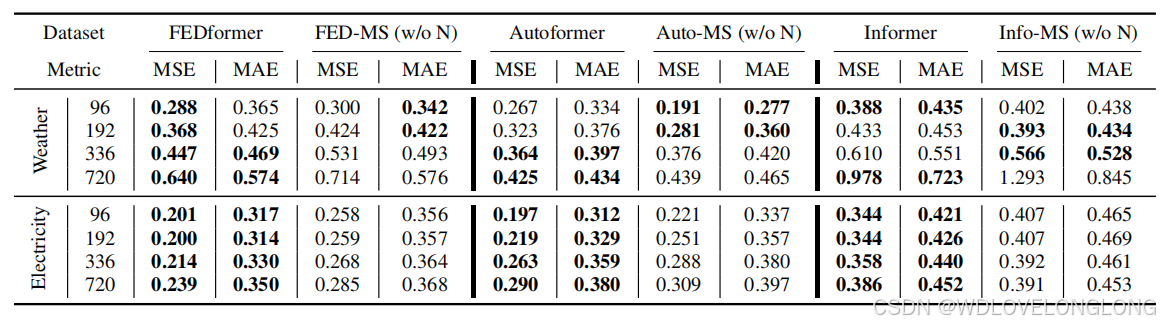
recorded influenza-like illness patients from the US Center for Disease Control and Prevention. We consider horizon lengths of 24, 32, 48, and 64 with an input length of 32.
Implementation details
: Following previous work (
Xu et al.
,
2021
;
Zhou et al.
,
2021
), we pass
X
enc
=
X
(
L
)
as the input to the encoder. While an array of zero-values would be the default to pass to the decoder, the decoder instead takes as input the second half of the look-back window padded with zeros X
dec
=
{
x
t
0
+
`
L
/
2
, ...,
x
`
L
,
0
,
0
, ...,
0
}
with length
`
L
/
2 +
`
H
. The hidden dimension of models is 512 with a batch size of 32. We use the Adam optimizer with a learning rate of 1e-4. The look-back window size is fixed to 96, and the horizon is varied from 96 to 720. We repeat each experiment 5 times and report average values to reduce randomness. For additional implementation details on our model and baselines please refer to Appendix
A
.
Main results and comparison with baselines
: Table
1
shows the results of the proposed framework compared to the baselines. Our proposed multi-scale framework with the adaptive loss outperforms the baselines in almost all of the experiments with an average improvement of 5
.
6%
over FEDFormer, 13% over Autoformer and
38%
over Informer which are the three most recent transformer-based architectures on MSE. We also achieved significant error reduction on MAE. The improvement is statistically significant in all cases, and in certain cases quite substantial. In particular for the exchange-rate dataset, with Informer and Reformer base models, our approach improves upon the respective baselines by over 50%
averaged over the different horizon lengths.
Time and memory complexity
: The proposed framework uses the same number of parameters for the model as the baselines (except two parameters α
and
c
of the Adaptive loss). Our framework sacri- fices a small amount of computation efficiency for the sake of a significant performance improvement. We expand our analysis in Appendix
C
. As shown in Table
4
in Appendix, if we replace the operation at the final scale by an interpolation of the prior output, we can achieve improved performance over the baselines, at no computational overhead.
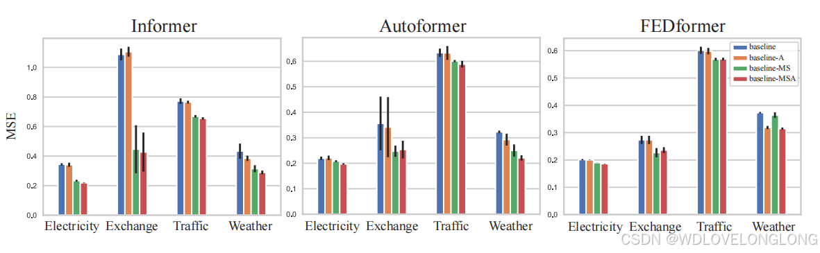
Figure 4: Comparison of training with Adaptive loss ”-
A
”, multi-scale framework with MSE loss
”-
MS
”, Multi-scale framework and Adaptive loss ”-
MSA
”. It shows the combination of all our
proposed contributions is essential, and results in significantly improved performance.
Table 3: Single-scale framework with cross scale normalization ”-
N
”. The cross-scale normalization (which in the single-scale case corresponds to mean-normalization of the output) does not improve the performance of the Autoformer, as it already has an internal trend-cycle normalization component. However, it does improve the results of the Informer and FEDformer.
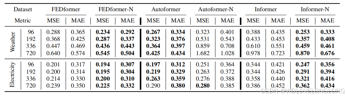
4.2 A
BLATION STUDY
We present main ablation studies in this section, more ablation results are shown in Appendix
G
.
Impact of each component
: Two important components of our approach are the multi-scale framework and the use of the adaptive loss. We conduct multiple experiments (1) removing the multi-scale framework and/or (2) replacing the Adaptive loss by the MSE for training, in order to demonstrate the benefits of these two components. Figure
4
shows the effect of multi-scale and the loss function with different base models. Considering the impact of ablating the adaptive loss, we can see that for both the multi-scale and base models, training with the adaptive loss improves performance. Similarly, adding the multi-scale framework improves performance, both with and without the adaptive loss. Overall, combining the adaptive loss with the multi-scale framework results in the best performance.
Cross-scale normalization
: As we discussed in Section
3.3
, having the cross-scale normalization is crucial to avoid the distribution shifts. To confirm that, we conduct two experiments. Firstly, we use the multi-scale framework without the cross-scale normalization to argue that the error accumulation and covariate shift between the scales leads higher error compared to only a single scale. As shown in Table
2
, while the multi-scale framework can get better results in a few cases, it mostly have higher errors than baselines. On the other hand, adding the normalization with only a single scale can still help to achieve better performance by reducing the effect of covariate shift between the training and the test series. As shown in Table
3
, the normalization improves the results of Informer and FEDformer consistently. The decomposition layer of the Autoformer solves a similar problem and replacing that with our normalization harms the capacity of the model.
4.3 Q
UALITATIVE
R
ESULTS
We have also shown the qualitative comparisons between the vanilla Informer and FEDformer
versus the results of our framework in Figure
5
. Most notably, in both cases our approach appears significantly better at forecasting the statistical properties (such as local variance) of the signal. Our scaleformer-based models capture trends (and other human-relevant) information better than their baselines. Despite these interesting findings, we would like to emphasize that these are randomly selected qualitative examples that may have their own limitations. For more qualitative results, please refer to Section
I
in the Appendix.
4.4 E
XTENSIONS AND
D
ISCUSSION
The Scaleformer structural prior has been shown to be beneficial when applied to transformer-based, deterministic time series forecasting. It is not however limited to those settings. In this section, we show it can be extended to probabilisitc forecasting
and non transformer-based encoders, both of which are closely coupled with our primary application. We also aim to highlight potential promising future directions.
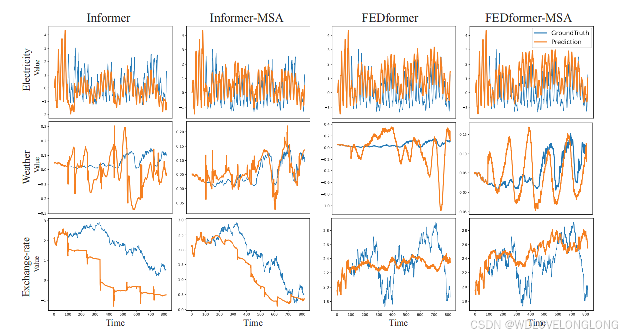
Figure 5: Qualitative comparison of base models with our framework. Our multi-scale models can
better capture the global trend and local variations of the signal than their baseline equivalents. To keep the figure concise and readable, we only show Informer and FEDformer, please refer to Figure
8
in Appendix for more results.
We show that our Scaleformer can improve performance in a probabilistic forecasting setting (please refer to Table
9
in Appendix for more details). We adopt the probabilistic output of DeepAR (
Salinas et al.
,
2020
), which is the most common probabilistic forecasting treatment. In this setting, instead of a point estimate, we have two prediction heads, predicting the mean µ
and standard deviation
σ
, trained with a negative log likelihood loss (NLL). NLL and continuous ranked probability score (CRPS) are used as evaluation metrics. All other hyperparameters remain unchanged. Here, again, scaleformers continue to outperform the probabilistic Informer.
While we have mainly focused on improving transformer-based models, they are not the only
encoders. Recent models such as NHits (
Challu et al.
,
2022
) and FiLM (
Zhou et al.
,
2022a
) attain
competitive performance, while assuming a fixed length univariate input/output. They are less flexible compared with variable length of multi-variate input/output, but result in strong performance and faster inference than transformers, making them interesting to consider. The Scaleformer prior demonstrates a statistically significant improvement, on average, when adapted by NHits and FiLM to iteratively refine predictions. For more details please refer to Appendix
K
. The results mentioned above demonstrate the fact that ScaleFormer can adapt to settings distinct from point-wise time-series forecasts with transformers (the primary scope of our paper), such as probabilistic forecasts and non-transformer models. We consider such directions to therefore be promising for future work.
5 C
ONCLUSION
Noting that introducing structural priors that account for multi-scale information is essential for
accurate time-series forecastings, this paper proposes a novel multi-scale framework on top of recent state-the-art methods for time-series forecasting using Transformers. Our framework iteratively refines a forecasted time-series at increasingly fine-grained scales, and introduces a normalization scheme that minimizes distribution shifts between scales. These contributions result in vastly improved performance over baseline transformer architectures, across a variety of settings, and qualitatively result in forecasts that better capture the trend and local variations of the target signal. Additionally, our detailed ablation study shows that the different components synergetically work together to deliver this outcome.


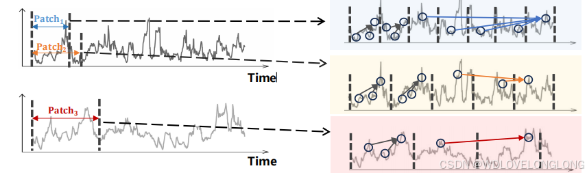
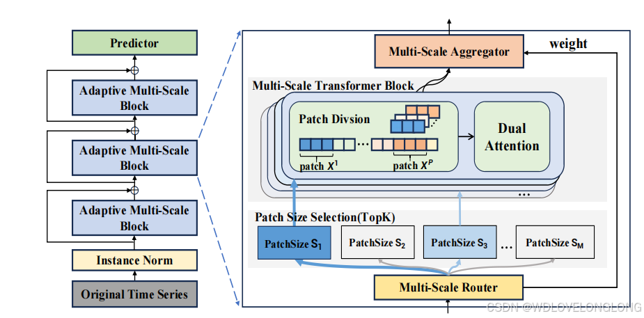
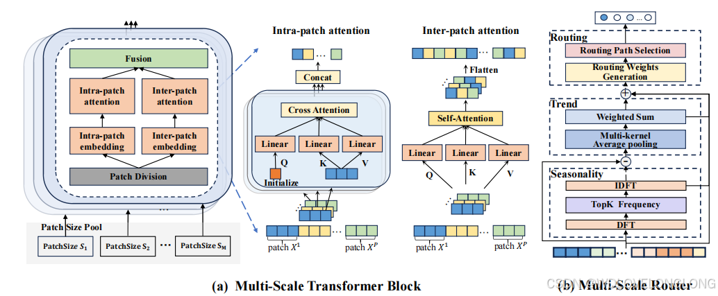


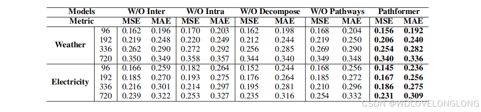

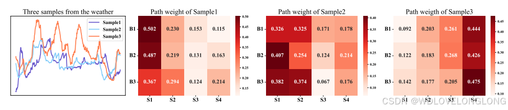


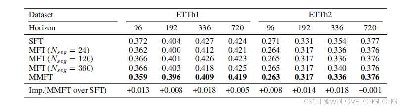
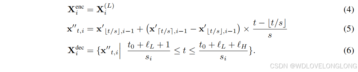
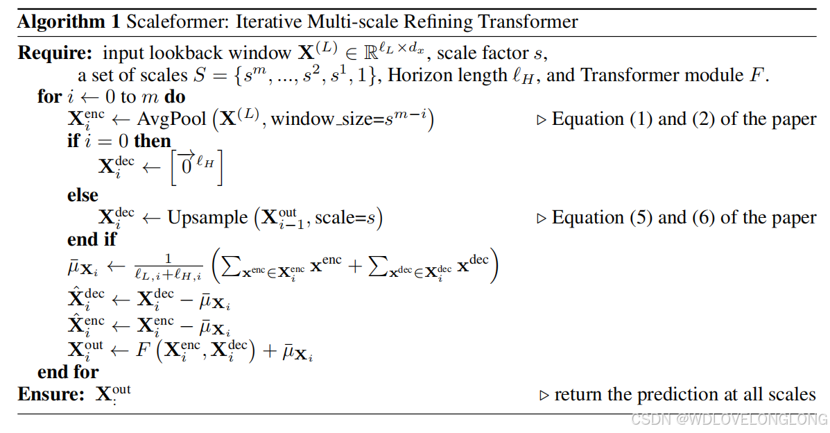

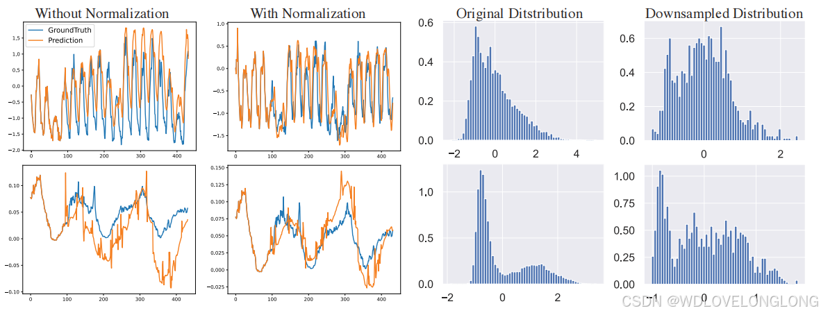
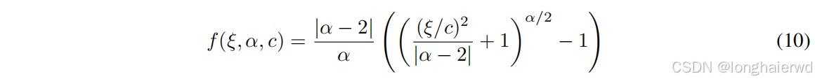
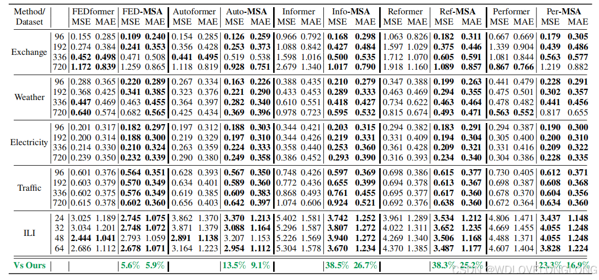


 1万+
1万+

 被折叠的 条评论
为什么被折叠?
被折叠的 条评论
为什么被折叠?
 到【灌水乐园】发言


