R语言笔记之线性回归及其衍生

普通线性回归

1.最小二乘线性模型

> dat=read.csv("https://raw.githubusercontent.com/happyrabbit/DataScientistR/master/Data/SegData.csv")
> dat=subset(dat,store_exp >0&online_exp >0)
> modeldat=dat[,grep("Q",names(dat))]
> modeldat$total_exp=dat$store_exp+dat$online_exp

下面展示输出结果，看哈数据是否有缺失值或离群点

> par(mfrow=c(1,2))
> hist(modeldat$total_exp,main="",xlab="total_exp")
> boxplot(modeldat$total_exp)
> 

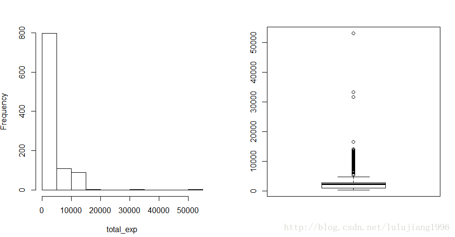
如上，数据集modeldat中没有缺失值，但是明显有离群点，而且因变量total_exp分布明显偏离正太。
我们需要删除离群点，然后对因变量进行对数变换
我们用Z分值的方法查找并删除离群点。

> y=modeldat$total_exp
 #求z分值
> zs=(y-mean(y))/mad(y)
 #找到z分值大于3.5的离群点，删除这些观测
> modeldat=modeldat[-which(zs>3.5),]
> 

接下来检查变量的共线性

> library(corrplot)
corrplot 0.84 loaded
Warning message:
程辑包‘corrplot’是用R版本3.4.3 来建造的 
> correlation=cor(modeldat[,grep("Q",names(modeldat))])
> corrplot.mixed(correlation,order="hclust",tl.pos="lt",upper="ellipse")

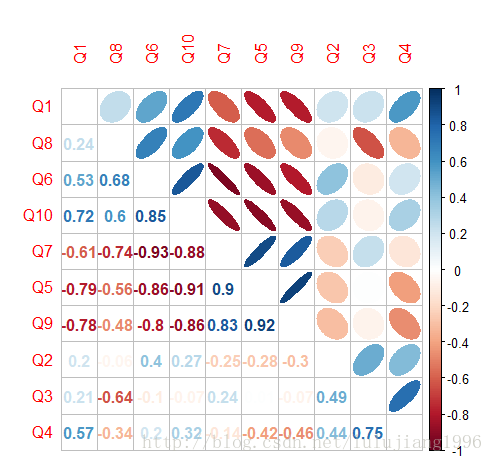
由上图可以看出，变量之间有很强的相关性。
我们需要删除高度相关变量的算法，设置阈值为0.75

> library(caret)
载入需要的程辑包：lattice
载入需要的程辑包：ggplot2
Warning messages:
1: 程辑包‘caret’是用R版本3.4.3 来建造的 
2: 程辑包‘lattice’是用R版本3.4.3 来建造的 
3: 程辑包‘ggplot2’是用R版本3.4.3 来建造的 
> highcor=findCorrelation(correlation,cutoff=.75)
> modeldat=modeldat[,-highcor]

现在我们可以拟合线性模型。“.“表示数据集modeldat中除了因变量外所有的变量都被当做自变量，这里我们没有考虑交互效应。
且我们对原始变量进行了对数变换

> limfit=lm(log(total_exp)~.,data=modeldat)
> summary(lmfit)
Error in summary(lmfit) : object 'lmfit' not found
> summary(limfit)

Call:
lm(formula = log(total_exp) ~ ., data = modeldat)

Residuals:
     Min       1Q   Median       3Q      Max 
-1.17494 -0.13719  0.01284  0.14163  0.56227 

Coefficients:
             Estimate Std. Error t value Pr(>|t|)    
(Intercept)  8.098314   0.054286 149.177  < 2e-16 ***
Q1          -0.145340   0.008823 -16.474  < 2e-16 ***
Q2           0.102275   0.019492   5.247 1.98e-07 ***
Q3           0.254450   0.018348  13.868  < 2e-16 ***
Q6          -0.227684   0.011520 -19.764  < 2e-16 ***
Q8          -0.090706   0.016497  -5.498 5.15e-08 ***
---
Signif. codes:  0 ‘***’ 0.001 ‘**’ 0.01 ‘*’ 0.05 ‘.’ 0.1 ‘ ’ 1

Residual standard error: 0.2262 on 805 degrees of freedom
Multiple R-squared:  0.8542,    Adjusted R-squared:  0.8533 
F-statistic: 943.4 on 5 and 805 DF,  p-value: