Real-Time Rendering——9.13.1 Filtering Normals and Normal Distributions过滤法线和正态分布

最新推荐文章于 2022-10-12 12:47:42 发布

椰子糖莫莫

最新推荐文章于 2022-10-12 12:47:42 发布

阅读量252

点赞数

分类专栏： Real-Time Rendering 文章标签：渲染管线

本文链接：https://blog.csdn.net/m0_37609239/article/details/126241139

版权

Real-Time Rendering 专栏收录该内容

102 篇文章 14 订阅

订阅专栏

The lion’s share of material filtering artifacts (primarily from specular aliasing), as well as the most frequently used solutions for them, are related to the filtering of normals and normal distribution functions. Because of its importance, we will discuss this aspect in some depth.

材质过滤伪像的最大部分(主要来自镜面混叠)，以及最常用的解决方案，都与法线和法线分布函数的过滤有关。因为它的重要性，我们将深入讨论这个方面。

To understand why these artifacts occur and how to solve them, recall that the NDF is a statistical description of subpixel surface structure. When the distance between the camera and surface increases, surface structures that previously covered multiple pixels may be reduced to subpixel size, moving from the realm of bump maps into the realm of the NDF. This transition is intimately tied to the mipmap chain,which encapsulates the reduction of texture details to subpixel size.

为了理解为什么会出现这些伪像以及如何解决它们，回想一下NDF是亚像素表面结构的统计描述。当相机和表面之间的距离增加时，先前覆盖多个像素的表面结构可以减小到子像素大小，从凹凸贴图的领域移动到NDF的领域。这种过渡与mipmap链密切相关，它封装了将纹理细节缩减为子像素大小的过程。

Consider how the appearance of an object, such as the cylinder at the left in Figure 9.49, is modeled for rendering. Appearance modeling always assumes a certain scale of observation. Macroscale (large-scale) geometry is modeled as triangles, mesoscale (middle-scale) geometry is modeled as textures, and microscale geometry, smaller than a single pixel, is modeled via the BRDF.

考虑一个物体的外观，比如图9.49中左边的圆柱体，是如何被建模以进行渲染的。外观建模总是假设一定的观察尺度。宏观尺度(大尺度)几何图形被建模为三角形，中尺度(中等尺度)几何图形被建模为纹理，而小于单个像素的微观尺度几何图形通过BRDF被建模。

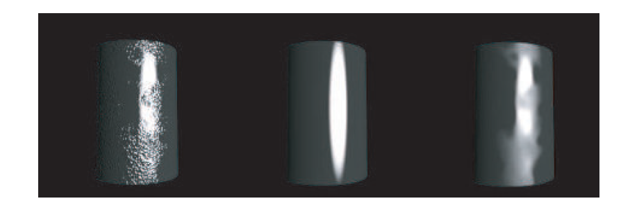
Figure 9.49. On the left, the cylinder is rendered with the original normal map. In the center, a much lower-resolution normal map containing averaged and renormalized normals is used, as shown in the bottom left of Figure 9.50. On the right, the cylinder is rendered with textures at the same low resolution, but containing normal and gloss values fitted to the ideal NDF, as shown in the bottom right of Figure 9.50. The image on the right is a significantly better representation of the original appearance. This surface will also be less prone to aliasing when rendered at low resolution. (Image courtesy of Patrick Conran, ILM.)

图9.49。在左侧，圆柱体使用原始法线贴图进行渲染。在中心，使用了一个分辨率低得多的法线贴图，包含了平均的和重正化的法线，如图9.50的左下方所示。在右边，圆柱体以同样低的分辨率渲染纹理，但是包含符合理想NDF的法线和光泽值，如图9.50的右下角所示。右边的图像更好地再现了原始外观。当以低分辨率渲染时，该表面也不容易出现锯齿。(图片由ILM的Patrick Conran提供。)

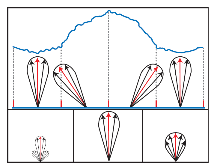
Figure 9.50. Part of the surface from Figure 9.49. The top row shows the normal distributions (the mean normal shown in red) and the implied microgeometry. The bottom row shows three ways to average the four NDFs into one, as done in mipmapping. On the left is the ground truth (averaging the normal distributions), the center shows the result of averaging the mean (normal) and variance (roughness) separately, and the right shows an NDF lobe fitted to the averaged NDF.

图9.50。图9.49中的部分表面。最上面一行显示了正态分布(平均正态显示为红色)和隐含的微观几何。底部一行显示了将四个NDF平均为一个的三种方法，如在mipmapping中所做的那样。左边是地面实况(对正态分布求平均)，中间显示分别对平均值(正态)和方差(粗糙度)求平均的结果，右边显示拟合到平均NDF的NDF波瓣。

Given the scale shown in the image, it is appropriate to model the cylinder as a smooth mesh (macroscale) and to represent the bumps with a normal map (mesoscale). A Beckmann NDF with a fixed roughness αb is chosen to model the microscale normal distribution. This combined representation models the cylinder appearance well at this scale. But, what happens when the scale of observation changes?

给定图像中显示的比例，将圆柱体建模为平滑网格(宏观尺度)并用法线贴图表示凸起(中尺度)是合适的。选择具有固定粗糙度αb的贝克曼NDF来模拟微尺度正态分布。这种组合表示在此比例下很好地模拟了圆柱体外观。但是，当观察范围改变时会发生什么呢？

Study Figure 9.50. The black-framed figure at the top shows a small part of the surface, covered by four normal-map texels. Assume that we are rendering the surface at a scale such that each normal map texel is covered by one pixel on average. For each texel, the normal (which is the average, or mean, of the distribution) is shown as a red arrow, surrounded by the Beckmann NDF, shown in black. The normals and NDF implicitly specify an underlying surface structure, shown in cross section. The large hump in the middle is one of the bumps from the normal map, and the small wiggles are the microscale surface structure. Each texel in the normal map, combined with the roughness, can be seen as collecting the distribution of normals across the surface area covered by the texel.

研究图9.50。顶部的黑框图显示了表面的一小部分，被四个法线贴图纹理元素覆盖。假设我们以一定的比例渲染表面，使得每个法线贴图纹理平均被一个像素覆盖。对于每个纹理元素，法线(分布的平均值)显示为红色箭头，被黑色显示的贝克曼NDF包围。法线和NDF隐含地指定了底层的表面结构，如横截面所示。中间的大驼峰是法线贴图中的一个凸起，小波浪是微尺度的表面结构。法线贴图中的每个纹理元素，结合粗糙度，可以被看作是在纹理元素覆盖的表面区域上收集法线的分布。

Now assume that the camera has moved further from the object, so that one pixel covers all four of the normal map texels. The ideal representation of the surface at this resolution would exactly represent the distribution of all normals collected across the larger surface area covered by each pixel. This distribution could be found by averaging the NDFs in the four texels of the top-level mipmap. The lower left figure shows this ideal normal distribution. This result, if used for rendering, would most accurately represent the appearance of the surface at this lower resolution.

现在假设相机已经远离物体，所以一个像素覆盖了所有四个法线贴图纹理像素。在此分辨率下，表面的理想表示将准确地表示在每个像素覆盖的较大表面区域上收集的所有法线的分布。这种分布可以通过对顶层小中见大贴图的四个纹理像素中的NDF进行平均来找到。左下图显示了这种理想的正态分布。如果用于渲染，此结果将最准确地表示较低分辨率下的表面外观。

The bottom center figure shows the result of separately averaging the normals, the mean of each distribution, and the roughness, which corresponds to the width of each. The result has the correct average normal (in red), but the distribution is too narrow. This error will cause the surface to appear too smooth. Worse, since the NDF is so narrow, it will tend to cause aliasing, in the form of flickering highlights.

底部中间的图显示了分别平均法线、每个分布的平均值和粗糙度(对应于每个分布的宽度)的结果。结果具有正确的平均正常值(红色)，但分布太窄。该错误将导致曲面看起来过于平滑。更糟糕的是，由于NDF太窄，它会以闪烁高光的形式导致混叠。

We cannot represent the ideal normal distribution directly with the Beckmann NDF. However, if we use a roughness map, the Beckmann roughness αb can be varied from texel to texel. Imagine that, for each ideal NDF, we find the oriented Beckmann lobe that matches it most closely, both in orientation and overall width. We store the center direction of this Beckmann lobe in the normal map, and its roughness value in the roughness map. The results are shown on the bottom right. This NDF is much closer to the ideal. The appearance of the cylinder can be represented much more faithfully with this process than with simple normal averaging, as can be seen in Figure 9.49.

我们不能用贝克曼NDF直接代表理想的正态分布。然而，如果我们使用粗糙度图，贝克曼粗糙度αb可以从一个纹理元素到另一个纹理元素变化。想象一下，对于每个理想的NDF，我们找到在方向和总宽度上与其最匹配的定向贝克曼瓣。我们将贝克曼叶的中心方向存储在法线贴图中，将其粗糙度值存储在粗糙度贴图中。结果显示在右下角。这个NDF更接近理想值。从图9.49中可以看出，用这种方法比用简单的正态平均法更能真实地表现圆柱体的外形。

For best results, filtering operations such as mipmapping should be applied to normal distributions, not normals or roughness values. Doing so implies a slightly different way to think about the relationship between the NDFs and the normals. Typically the NDF is defined in the local tangent space determined by the normal map’s per-pixel normal. However, when filtering NDFs across different normals, it is more useful to think of the combination of the normal map and roughness map as defining a skewed NDF (one that does not average to a normal pointing straight up) in the tangent space of the underlying geometrical surface.

为了获得最佳效果，过滤操作(如mipmapping)应该应用于法线分布，而不是法线或粗糙度值。这样做意味着以稍微不同的方式思考NDF和法线之间的关系。通常，NDF在由法线贴图的每像素法线确定的局部切线空间中定义。但是，在过滤不同法线的NDF时，更有用的做法是将法线贴图和粗糙度贴图的组合视为在基础几何曲面的切线空间中定义一个倾斜的NDF(不是垂直指向法线的NDF)。

Early attempts to solve the NDF filtering problem [91, 284, 658] used numerical optimization to fit one or more NDF lobes to the averaged distribution. This approach suffers from robustness and speed issues, and is not used much today. Instead, most techniques currently in use work by computing the variance of the normal distribution. Toksvig [1774] makes a clever observation that if normals are averaged and not renormalized, the length of the averaged normal correlates inversely with the width of the normal distribution. That is, the more the original normals point in different directions, the shorter the normal averaged from them. He presents a method to modify the NDF roughness parameter based on this normal length. Evaluating the BRDF with the modified roughness approximates the spreading effect of the filtered normals.

解决NDF滤波问题的早期尝试[91，284，658]使用数值优化将一个或多个NDF波瓣拟合到平均分布。这种方法存在鲁棒性和速度问题，现在已经不怎么使用了。相反，目前使用的大多数技术是通过计算正态分布的方差来工作的。Toksvig [1774]做了一个巧妙的观察，如果法线被平均并且没有重正化，平均法线的长度与法线分布的宽度成反比。也就是说，原始法线指向不同的方向越多，从它们平均得到的法线就越短。他提出了一种基于该法向长度来修改NDF粗糙度参数的方法。用修改的粗糙度评估BRDF近似于过滤法线的扩散效果。

Toksvig’s original equation was intended for use with the Blinn-Phong NDF:

Toksvig的原始方程旨在用于Blinn-Phong NDF:

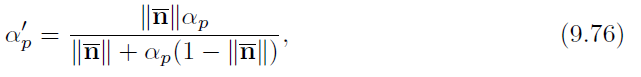
where αp is the original roughness parameter value, α′p is the modified value, and is the length of the averaged normal. The equation can also be used with the Beckmann NDF by applying the equivalence (fromWalter et al. [1833]),since the shapes of the two NDFs are quite close. Using the method with GGX is less straightforward, since there is no clear equivalence between GGX and Blinn-Phong (or Beckmann). Using the αb equivalence for αg gives the same value at the center of the highlight, but the highlight appearance is quite different. More troubling, the variance of the GGX distribution is undefined, which puts this variance-based family of techniques on shaky theoretical ground when used with GGX. Despite these theoretical difficulties, it is fairly common to use Equation 9.76 with the GGX distribution, typically using . Doing so works reasonably well in practice.

其中，αp是原始粗糙度参数值，α′p是修正值，是平均法线的长度。由于两种NDF的形状非常接近，通过应用等价关系(fromWalter等人[1833])，该方程也可用于Beckmann NDF。用GGX的方法就不那么简单了，因为在GGX和Blinn-Phong(或Beckmann)之间没有明确的等价关系。对αg使用αb等价会在高光的中心给出相同的值，但是高光的外观会有很大的不同。更麻烦的是，GGX分布的方差是不确定的，这使得这种基于方差的技术在与GGX一起使用时，其理论基础摇摇欲坠。尽管存在这些理论上的困难，但将方程9.76与GGX分布结合使用还是很常见的，通常使用。这样做在实践中相当有效。

Toksvig’s method has the advantage of accounting for normal variance introduced by GPU texture filtering. It also works with the simplest normal mipmapping scheme, linear averaging without normalization. This feature is particularly useful for dynamically generated normal maps such as water ripples, for which mipmap generation must be done on the fly. The method is not as good for static normal maps, since it does not work well with prevailing methods of compressing normal maps. These compression methods rely on the normal being of unit length. Since Toksvig’s method relies on the length of the average normal varying, normal maps used with it may have to remain uncompressed. Even then, storing the shortened normals can result in precision issues.

Toksvig的方法具有解决由GPU纹理过滤引入的正态方差的优势。它还可以与最简单的正常小中见大贴图方案(无归一化的线性平均)一起工作。此功能对于动态生成的法线贴图(如水波纹)特别有用，因为它的mipmap生成必须在运行中完成。该方法不适合静态法线贴图，因为它不适合压缩法线贴图的流行方法。这些压缩方法依赖于单位长度的标准长度。由于Toksvig的方法依赖于平均法线变化的长度，因此与其一起使用的法线贴图可能必须保持未压缩。即使这样，存储缩短的法线也会导致精度问题。

Olano and Baker’s LEAN mapping technique [1320] is based on mapping the covariance matrix of the normal distribution. Like Toksvig’s technique, it works well with GPU texture filtering and linear mipmapping. It also supports anisotropic normal distributions. Similarly to Toksvig’s method, LEAN mapping works well with dynamically generated normals, but to avoid precision issues, it requires a large amount of storage when used with static normals. A similar technique was independently developed by Hery et al. [731, 732] and used in Pixar’s animated films to render subpixel details such as metal flakes and small scratches. A simpler variant of LEAN mapping, CLEAN mapping [93], requires less storage at the cost of losing anisotropy support. LEADR mapping [395, 396] extends LEAN mapping to also account for the visibility effects of displacement mapping.

Olano和Baker的精益映射技术[1320]基于映射正态分布的协方差矩阵。像Toksvig的技术一样，它与GPU纹理过滤和线性mipmapping配合得很好。它还支持各向异性正态分布。与Toksvig的方法类似，精益贴图适用于动态生成的法线，但为了避免精度问题，当用于静态法线时，它需要大量的存储。张国晖等人[731，732]独立开发了一种类似的技术，并用于皮克斯的动画电影中，以渲染金属薄片和小划痕等亚像素细节。精益映射的一个更简单的变体，干净映射[93]，需要更少的存储，代价是失去各向异性支持。LEADR映射[395，396]扩展了精益映射，也考虑了位移映射的可见性影响。

The majority of normal maps used in real-time applications are static, rather than dynamically generated. For such maps, the variance mapping family of techniques is commonly used. In these techniques, when the normal map’s mipmap chain is generated, the variance that was lost through averaging is computed. Hill [739] notes that the mathematical formulations of Toksvig’s technique, LEAN mapping, and CLEAN mapping could each be used to precompute variance in this way, which removes many of the disadvantages of these techniques when used in their original forms. In some cases the precomputed variance values are stored in the mipmap chain of a separate variance texture. More often, these values are used to modify the mipmap chain of an existing roughness map. For example, this method is employed in the variancemapping technique used in the game Call of Duty: Black Ops [998]. The modified roughness values are computed by converting the original roughness values to variance values, adding in the variance from the normal map, and converting the result back to roughness. For the game The Order: 1886, Neubelt and Pettineo [1266, 1267] use a technique by Han [658] in a similar way. They convolve the normal map NDF with the NDF of their BRDF’s specular term, convert the result to roughness, and store it in a roughness map.

实时应用中使用的大多数法线贴图是静态的，而不是动态生成的。对于这样的地图，方差映射技术族是常用的。在这些技术中，当法线贴图的小中见大贴图链被生成时，通过平均丢失的方差被计算。Hill [739]指出，Toksvig技术的数学公式、精益映射和干净映射都可以用于以这种方式预计算方差，这消除了这些技术以原始形式使用时的许多缺点。在某些情况下，预计算的方差值存储在单独的方差纹理的小中见大贴图链中。更常见的是，这些值用于修改现有粗糙度贴图的中值贴图链。例如，游戏《使命召唤:黑色行动[998]》中使用的变量映射技术就采用了这种方法。通过将原始粗糙度值转换为方差值，加上来自法线贴图的方差，并将结果转换回粗糙度，来计算修改的粗糙度值。在游戏《秩序:1886》中，纽贝尔特和佩提尼奥[1266，1267]以类似的方式使用了韩[658]的技巧。他们将法线贴图NDF与BRDF的镜面反射项的NDF进行卷积，将结果转换为粗糙度，并将其存储在粗糙度贴图中。

For improved results at the cost of some extra storage, variance can be computed in the texture-space x- and y-directions and stored in an anisotropic roughness map [384, 740, 1823]. By itself this technique is limited to axis-aligned anisotropy, which is typical in man-made surfaces but less so in naturally occurring ones. At the cost of storing one more value, oriented anisotropy can be supported as well [740].

为了以一些额外存储为代价改善结果，可以在纹理空间x和y方向上计算方差，并存储在各向异性粗糙度图中[384，740，1823]。就其本身而言，这种技术仅限于轴向排列的各向异性，这在人造表面中很典型，但在自然发生的表面中不太常见。以多存储一个值为代价，也可以支持定向各向异性[740]。

Unlike the original forms of Toksvig, LEAN, and CLEAN mapping, variance mapping techniques do not account for variance introduced by GPU texture filtering. To compensate for this, variance mapping implementations often convolve the top-level mip of the normal map with a small filter [740, 998]. When combining multiple normal maps, e.g., detail normal mapping [106], care needs to be taken to combine the variance of the normal maps correctly [740, 960].

与Toksvig、LEAN和CLEAN贴图的原始形式不同，方差贴图技术不考虑GPU纹理过滤引入的方差。为了弥补这一点，方差映射实现通常用一个小滤波器对法线映射的顶层mip进行卷积[740，998]。当组合多个法线映射时，例如，细节法线映射[106]，需要注意正确地组合法线映射的方差[740，960]。

Normal variance can be introduced by high-curvature geometry as well as normal maps. Artifacts resulting from this variance are not mitigated by the previously discussed techniques. A different set of methods exists to address geometry normal variance. If a unique texture mapping exists over the geometry (often the case with characters, less so with environments) then the geometry curvature can be “baked” into the roughness map [740]. The curvature can also be estimated on the fly, using pixel-shader derivative instructions [740, 857, 1229, 1589, 1775, 1823]. This estimation can be done when rendering the geometry, or in a post-process pass, if a normal buffer is available.

法线方差可以由高曲率几何以及法线贴图引入。由这种差异产生的伪像不能通过前面讨论的技术来减轻。存在一组不同的方法来解决几何正态方差。如果在几何图形上存在唯一的纹理映射(通常是字符的情况，较少是环境的情况)，那么几何图形曲率可以被“烘焙”到粗糙度映射中[740]。曲率也可以使用像素着色器衍生指令[740，857，1229，1589，1775，1823]来动态估计。如果正常缓冲区可用，可以在渲染几何图形时或在后处理过程中进行此估计。

The approaches discussed so far focus on specular response, but normal variance can affect diffuse shading as well. Taking account of the effect of normal variance on the n · l term can help increase accuracy of both diffuse and specular shading since both are multiplied by this factor in the reflectance integral [740].

到目前为止，讨论的方法主要集中在镜面反射上，但是法线变化也会影响漫反射着色。考虑正态方差对n · l项的影响有助于提高漫反射和镜面反射阴影的精确度，因为两者都在反射积分中乘以该因子【740】。

Variance mapping techniques approximate the normal distribution as a smooth Gaussian lobe. This is a reasonable approximation if every pixel covers hundreds of thousands of bumps, so that they all average out smoothly. However, in many cases a pixel many cover only a few hundred or a few thousand bumps, which can lead to a “glinty” appearance. An example of this can be seen in Figure 9.25 on page 328, which is a sequence of images showing a sphere with bumps that diminish in size from image to image. The bottom right image shows the result when the bumps are small enough to average into a smooth highlight, but the images on the bottom left and bottom center show bumps that are smaller than a pixel but not small enough to average smoothly. If you were to observe an animated rendering of these spheres, the noisy highlight would appear as glints that sparkle in and out from frame to frame.

方差映射技术将正态分布近似为平滑的高斯波瓣。如果每个像素都覆盖了成千上万个凸起，那么这是一个合理的近似值，这样它们就能平滑地达到平均。然而，在许多情况下，一个像素可能只覆盖几百或几千个凸起，这可能导致“闪烁”的外观。这方面的一个例子可以在328页的图9.25中看到，这是一系列图像，显示了一个带有凸起的球体，这些凸起的尺寸随着图像的不同而减小。右下方的图像显示了当凸起小到足以平均为平滑高光时的结果，但左下方和底部中间的图像显示了小于一个像素但不足以平滑平均的凸起。如果你观察这些球体的动画渲染，嘈杂的高光会以闪烁的形式出现，从一帧到另一帧闪烁。

If we were to plot the NDF of such a surface, it would look like the left image in Figure 9.51. As the sphere animates, the h vector moves over the NDF and crosses over bright and dark areas, which causes the “sparkly” appearance. If we were to use variance mapping techniques on this surface, it would effectively approximate this NDF with a smooth NDF similar to the one on the right of Figure 9.51, losing the sparkly details.

如果我们画出这样一个表面的NDF，它看起来像图9.51中的左图。当球体激活时，h向量在NDF上移动并穿过明亮和黑暗的区域，这导致了“闪闪发光”的外观。如果我们在这个表面上使用方差映射技术，它将有效地用一个类似于图9.51右边的平滑的NDF来近似这个NDF，失去了闪光的细节。

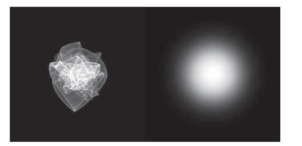
Figure 9.51. On the left is the NDF of a small patch (a few dozen bumps on a side) of a random bumpy surface. On the right is a Beckmann NDF lobe of approximately the same width. (Image courtesy of Miloˇs Haˇsan.)

图9.51。左侧是随机凹凸表面的一小块(一侧有几十个凸起)的NDF。右边是一个宽度大致相同的贝克曼NDF瓣。(图片由Milos Hasan提供。)

In the film industry this is often solved with extensive supersampling, which is not feasible in real-time rendering applications and undesirable even in offline rendering.Several techniques have been developed to address this issue. Some are unsuitable for real-time use, but may suggest avenues for future research [84, 810, 1941, 1942]. Two techniques have been designed for real-time implementation. Wang and Bowles [187, 1837] present a technique that is used to render sparkling snow in the game Disney Infinity 3.0. The technique aims to produce a plausible sparkly appearance rather than simulating a particular NDF. It is intended for use on materials such as snow that have relatively sparse sparkles. Zirr and Kaplanyan’s technique [1974] simulates normal distributions on multiple scales, is spatially and temporally stable, and allows for a wider variety of appearances.

在电影工业中，这通常通过大量的超级采样来解决，这在实时渲染应用中是不可行的，甚至在离线渲染中也是不期望的。已经开发了几种技术来解决这个问题。有些不适合实时使用，但可能为未来的研究提供途径[84，810，1941，1942]。已经为实时实现设计了两种技术。王和鲍尔斯[187，1837]提出了一种技术，用于渲染游戏迪士尼无限3.0闪闪发光的雪。该技术旨在产生一种看似可信的闪亮外观，而不是模拟特定的NDF。它旨在用于具有相对稀疏火花的材质，如雪。Zirr和Kaplanyan的技术[1974]模拟了多个尺度上的正态分布，在空间和时间上是稳定的，并允许更广泛的外观变化。

We do not have space to cover all of the extensive literature on material filtering, so we will mention a few notable references. Bruneton et al. [204] present a technique for handling variance on ocean surfaces across scales from geometry to BRDF, including environment lighting. Schilling [1565] discusses a variance mapping-like technique that supports anisotropic shading with environment maps. Bruneton and Neyret [205] provide a thorough overview of earlier work in this area.

我们没有足够的空间来涵盖所有关于材料过滤的大量文献，因此我们将提到一些值得注意的参考文献。Bruneton等人[204]提出了一种技术，用于处理从几何到BRDF范围内海洋表面的变化，包括环境照明。Schilling [1565]讨论了一种支持环境贴图各向异性着色的类似方差贴图的技术。Bruneton和Neyret [205]对该领域的早期工作进行了全面概述。