Python机器学习---比较基于小规模数据集的不同簇算法

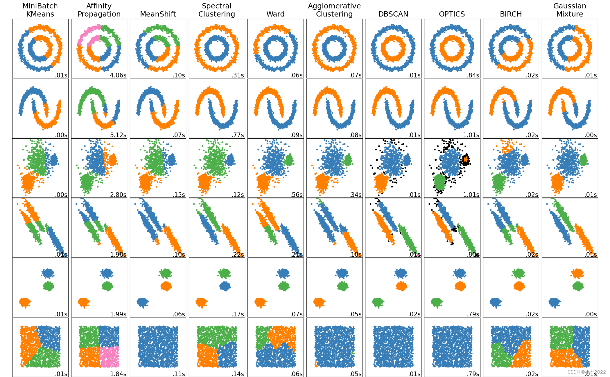
This example shows characteristics of different clustering algorithms on datasets that are “interesting” but still in 2D. With the exception of the last dataset, the parameters of each of these dataset-algorithm pairs has been tuned to produce good clustering results. Some algorithms are more sensitive to parameter values than others.

The last dataset is an example of a ‘null’ situation for clustering: the data is homogeneous, and there is no good clustering. For this example, the null dataset uses the same parameters as the dataset in the row above it, which represents a mismatch in the parameter values and the data structure.

While these examples give some intuition about the algorithms, this intuition might not apply to very high dimensional data.

import time
import warnings

import numpy as np
import matplotlib.pyplot as plt

from sklearn import cluster, datasets, mixture
from sklearn.neighbors import kneighbors_graph
from sklearn.preprocessing import StandardScaler
from itertools import cycle, islice

np.random.seed(0)

# ============
# Generate datasets. We choose the size big enough to see the scalability
# of the algorithms, but not too big to avoid too long running times
# ============
n_samples = 1500
noisy_circles = datasets.make_circles(n_samples=n_samples, factor=0.5, noise=0.05)
noisy_moons = datasets.make_moons(n_samples=n_samples, noise=0.05)
blobs = datasets.make_blobs(n_samples=n_samples, random_state=8)
no_structure = np.random.rand(n_samples, 2), None

# Anisotropicly distributed data
random_state = 170
X, y = datasets.make_blobs(n_sa