


背景:运行sklearn的谱聚类代码时候,需要对代码进行参数设定。并且聚类每次结果都不一样。所以需要深入算法底层,弄清楚算法怎么工作的,以及每个参数的意义。
源码地址:https://github.com/scikit-learn/scikit-learn/blob/7b136e9/sklearn/cluster/spectral.py#L275
算法及原理:Graph特征提取方法:谱聚类(Spectral Clustering)详解
目录
Comparing different clustering algorithms on toy datasets
一、输入参数
需要弄懂原理之后才能看懂相应的输入参数。Graph特征提取方法:谱聚类(Spectral Clustering)详解
1.1 聚类组数
n_clusters : integer, optional聚类后的聚类的group数,也就是原理中的k。
The dimension of the projection subspace.
也叫图分割,相当于把一个图分成许多个子图。

一个图G可能有很多个子图Gi(总共k个),子图之间没有交集。但是所有子图并在一起得到图G
简而言之,就是图分割成子图之后,分割不重不漏: Gi∩Gj=∅,且G1∪G2∪...∪Gk=G,
1.2 向量分解
eigen_solver : {None, ‘arpack’, ‘lobpcg’, or ‘amg’}
向量运算的算法,用于向量分解。
The eigenvalue decomposition strategy to use. AMG requires pyamg to be installed. It can be faster on very large, sparse problems, but may also lead to instabilities
eigen_tol : float, optional, default: 0.0求得拉普拉斯矩阵的时候的求解器的方法。很多种。
Stopping criterion for eigendecomposition of the Laplacian matrix when using arpack eigen_solver.
1.3 对矩阵H的操作
对矩阵H的操作
assign_labels : {‘kmeans’, ‘discretize’}, default: ‘kmeans’可以kmeans,也可以discretize
The strategy to use to assign labels in the embedding space. There are two ways to assign labels after the laplacian embedding. k-means can be applied and is a popular choice. But it can also be sensitive to initialization. Discretization is another approach which is less sensitive to random initialization.
k-means直接被运用起来,即对原理中的指引向量H中的行进行聚类。
原理:
聚类的时候,分别对H中的行进行聚类即可,通常是kmeans,也可以是GMM,具体看效果而定。
所以问题的转换是这样的:图聚类——切图——求最小化cut——求最小化cut对应的指引向量H
random_state : int, RandomState instance or None (default)
初始化的种子,伪随机数,用于K-means聚类的初始化。
A pseudo random number generator used for the initialization of the lobpcg eigen vectors decomposition when eigen_solver == ‘amg’ and by the K-Means initialization. Use an int to make the randomness deterministic. See Glossary.
n_init : int, optional, default: 10
K-means的中心种子数
Number of time the k-means algorithm will be run with different centroid seeds. The final results will be the best output of n_init consecutive runs in terms of inertia.
1.4 距离函数W
这里的参数跟距函数有关,这部分参数关于子图中的W

- Gi与
 互为补集合
互为补集合 - C()表示cost函数,
 表示第i个子图与其补集之间的cost
 - 整个分割的cost表示为所有分割后的子图与其补集合之间cost的和
- C(G1,G2)表示子图G1和子图G2的cost为两图之间所有节点的w
高斯核函数:
直接用高斯核函数作为距离,


- 表示样本点之间的相似度w直接用高斯核函数的距离表示
- σ表示样本点的邻域宽度,σ越大则w越大,即样本点之间的相似度越大
- 可以参考右图,σ可以看做半径,σ越大则对于同一个点的高度越高即w越大,越相近
gamma : float, default=1.0
如果用k近邻法,则此参数无用。是高斯核函数的中心值,可能是σ
Kernel coefficient for rbf, poly, sigmoid, laplacian and chi2 kernels. Ignored for affinity='nearest_neighbors'.
1.5 求得W的方法
affinity : string, array-like or callable, default ‘rbf’
If a string, this may be one of ‘nearest_neighbors’, ‘precomputed’, ‘rbf’ or one of the kernels supported by sklearn.metrics.pairwise_kernels.
Only kernels that produce similarity scores (non-negative values that increase with similarity) should be used. This property is not checked by the clustering algorithm.
如果nearest_neighbors参数,是就K近邻法(k近邻法k-nearest nerghbor),具体看原理:

或者

n_neighbors : integer,这个参数在选用k近邻法时候会用的,选用RBF忽略
Number of neighbors to use when constructing the affinity matrix using the nearest neighbors method. Ignored for affinity='rbf'.
如果RBF参数,就是下面这样:也称为全连接法(fully connected graph),径向基函数 (Radial Basis Function 简称 RBF)
如果precomputed:
这点需要弄懂,即可以指定相似矩阵。
1.6 kernels相关
这部分暂时没在原理之中找到对应,我们需要再详细研究。
degree : float, default=3
Degree of the polynomial kernel. Ignored by other kernels.
coef0 : float, default=1
Zero coefficient for polynomial and sigmoid kernels. Ignored by other kernels.
kernel_params : dictionary of string to any, optional
Parameters (keyword arguments) and values for kernel passed as callable object. Ignored by other kernels.
1.7 并行性
n_jobs : int or None, optional (default=None)
The number of parallel jobs to run. None means 1 unless in a joblib.parallel_backend context. -1 means using all processors. See Glossary for more details.
二、附属输入
2.1 affinity matrix
affinity_matrix_rray-like, shape (n_samples, n_samples)
adjacent matrix和affinity matrix之间的区别,一个是点与点之间的关系,一个是点与边之间的关系。
这个是否表示节点与边之间的关系?这个需要仔细查阅源码之后才能确定。
https://blog.csdn.net/songkun123/article/details/80720938
Affinity matrix used for clustering. Available only if after calling fit.
2.2 labels_
Labels of each point每个节点的label
三、关于affinity matrix
adjacent matrix表示点与点之间的关系,affinity matrix表示点与边之间的关系。
用法:
pred_y = SpectralClustering(n_clusters=2,random_state=1,affinity='precomputed').fit_predict(sub_correlation_matrix)
Examples
>>>
>>> from sklearn.cluster import SpectralClustering
>>> import numpy as np
>>> X = np.array([[1, 1], [2, 1], [1, 0],
...               [4, 7], [3, 5], [3, 6]])
>>> clustering = SpectralClustering(n_clusters=2,
...         assign_labels="discretize",
...         random_state=0).fit(X)
>>> clustering.labels_
array([1, 1, 1, 0, 0, 0])
>>> clustering
SpectralClustering(affinity='rbf', assign_labels='discretize', coef0=1,
          degree=3, eigen_solver=None, eigen_tol=0.0, gamma=1.0,
          kernel_params=None, n_clusters=2, n_init=10, n_jobs=None,
          n_neighbors=10, random_state=0)
Methods
fit(self, X[, y]) | Creates an affinity matrix for X using the selected affinity, then applies spectral clustering to this affinity matrix. |
fit_predict(self, X[, y]) | Performs clustering on X and returns cluster labels. |
get_params(self[, deep]) | Get parameters for this estimator. |
set_params(self, \*\*params) | Set the parameters of this estimator. |
__init__(self, n_clusters=8, eigen_solver=None, random_state=None, n_init=10, gamma=1.0, affinity=’rbf’, n_neighbors=10, eigen_tol=0.0, assign_labels=’kmeans’, degree=3, coef0=1, kernel_params=None, n_jobs=None)[source]
fit(self, X, y=None)[source]
Creates an affinity matrix for X using the selected affinity, then applies spectral clustering to this affinity matrix.
| Parameters: | X : array-like or sparse matrix, shape (n_samples, n_features) OR, if affinity==`precomputed`, a precomputed affinity matrix of shape (n_samples, n_samples) y : Ignored |
|---|
fit_predict(self, X, y=None)[source]
Performs clustering on X and returns cluster labels.
| Parameters: | X : ndarray, shape (n_samples, n_features) Input data. y : Ignored not used, present for API consistency by convention. |
|---|---|
| Returns: | labels : ndarray, shape (n_samples,) cluster labels |
get_params(self, deep=True)[source]
Get parameters for this estimator.
| Parameters: | deep : boolean, optional If True, will return the parameters for this estimator and contained subobjects that are estimators. |
|---|---|
| Returns: | params : mapping of string to any Parameter names mapped to their values. |
set_params(self, **params)[source]
Set the parameters of this estimator.
The method works on simple estimators as well as on nested objects (such as pipelines). The latter have parameters of the form <component>__<parameter> so that it’s possible to update each component of a nested object.
| Returns: | self |
|---|
四、例程
Comparing different clustering algorithms on toy datasets
This example shows characteristics of different clustering algorithms on datasets that are “interesting” but still in 2D. With the exception of the last dataset, the parameters of each of these dataset-algorithm pairs has been tuned to produce good clustering results. Some algorithms are more sensitive to parameter values than others.
The last dataset is an example of a ‘null’ situation for clustering: the data is homogeneous, and there is no good clustering. For this example, the null dataset uses the same parameters as the dataset in the row above it, which represents a mismatch in the parameter values and the data structure.
While these examples give some intuition about the algorithms, this intuition might not apply to very high dimensional data.
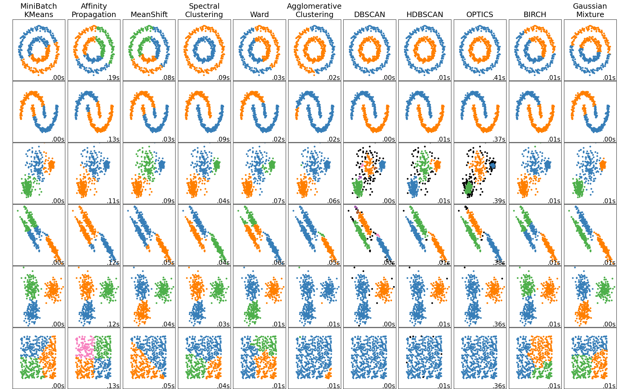
print(__doc__)

import time
import warnings

import numpy as np
import matplotlib.pyplot as plt

from sklearn import cluster, datasets, mixture
from sklearn.neighbors import kneighbors_graph
from sklearn.preprocessing import StandardScaler
from itertools import cycle, islice

np.random.seed(0)

# ============
# Generate datasets. We choose the size big enough to see the scalability
# of the algorithms, but not too big to avoid too long running times
# ============
n_samples = 1500
noisy_circles = datasets.make_circles(n_samples=n_samples, factor=.5,
                                      noise=.05)
noisy_moons = datasets.make_moons(n_samples=n_samples, noise=.05)
blobs = datasets.make_blobs(n_samples=n_samples, random_state=8)
no_structure = np.random.rand(n_samples, 2), None

# Anisotropicly distributed data
random_state = 170
X, y = datasets.make_blobs(n_samples=n_samples, random_state=random_state)
transformation = [[0.6, -0.6], [-0.4, 0.8]]
X_aniso = np.dot(X, transformation)
aniso = (X_aniso, y)

# blobs with varied variances
varied = datasets.make_blobs(n_samples=n_samples,
                             cluster_std=[1.0, 2.5, 0.5],
                             random_state=random_state)

# ============
# Set up cluster parameters
# ============
plt.figure(figsize=(9 * 2 + 3, 12.5))
plt.subplots_adjust(left=.02, right=.98, bottom=.001, top=.96, wspace=.05,
                    hspace=.01)

plot_num = 1

default_base = {'quantile': .3,
                'eps': .3,
                'damping': .9,
                'preference': -200,
                'n_neighbors': 10,
                'n_clusters': 3,
                'min_samples': 20,
                'xi': 0.05,
                'min_cluster_size': 0.1}

datasets = [
    (noisy_circles, {'damping': .77, 'preference': -240,
                     'quantile': .2, 'n_clusters': 2,
                     'min_samples': 20, 'xi': 0.25}),
    (noisy_moons, {'damping': .75, 'preference': -220, 'n_clusters': 2}),
    (varied, {'eps': .18, 'n_neighbors': 2,
              'min_samples': 5, 'xi': 0.035, 'min_cluster_size': .2}),
    (aniso, {'eps': .15, 'n_neighbors': 2,
             'min_samples': 20, 'xi': 0.1, 'min_cluster_size': .2}),
    (blobs, {}),
    (no_structure, {})]

for i_dataset, (dataset, algo_params) in enumerate(datasets):
    # update parameters with dataset-specific values
    params = default_base.copy()
    params.update(algo_params)

    X, y = dataset

    # normalize dataset for easier parameter selection
    X = StandardScaler().fit_transform(X)

    # estimate bandwidth for mean shift
    bandwidth = cluster.estimate_bandwidth(X, quantile=params['quantile'])

    # connectivity matrix for structured Ward
    connectivity = kneighbors_graph(
        X, n_neighbors=params['n_neighbors'], include_self=False)
    # make connectivity symmetric
    connectivity = 0.5 * (connectivity + connectivity.T)

    # ============
    # Create cluster objects
    # ============
    ms = cluster.MeanShift(bandwidth=bandwidth, bin_seeding=True)
    two_means = cluster.MiniBatchKMeans(n_clusters=params['n_clusters'])
    ward = cluster.AgglomerativeClustering(
        n_clusters=params['n_clusters'], linkage='ward',
        connectivity=connectivity)
    spectral = cluster.SpectralClustering(
        n_clusters=params['n_clusters'], eigen_solver='arpack',
        affinity="nearest_neighbors")
    dbscan = cluster.DBSCAN(eps=params['eps'])
    optics = cluster.OPTICS(min_samples=params['min_samples'],
                            xi=params['xi'],
                            min_cluster_size=params['min_cluster_size'])
    affinity_propagation = cluster.AffinityPropagation(
        damping=params['damping'], preference=params['preference'])
    average_linkage = cluster.AgglomerativeClustering(
        linkage="average", affinity="cityblock",
        n_clusters=params['n_clusters'], connectivity=connectivity)
    birch = cluster.Birch(n_clusters=params['n_clusters'])
    gmm = mixture.GaussianMixture(
        n_components=params['n_clusters'], covariance_type='full')

    clustering_algorithms = (
        ('MiniBatchKMeans', two_means),
        ('AffinityPropagation', affinity_propagation),
        ('MeanShift', ms),
        ('SpectralClustering', spectral),
        ('Ward', ward),
        ('AgglomerativeClustering', average_linkage),
        ('DBSCAN', dbscan),
        ('OPTICS', optics),
        ('Birch', birch),
        ('GaussianMixture', gmm)
    )

    for name, algorithm in clustering_algorithms:
        t0 = time.time()

        # catch warnings related to kneighbors_graph
        with warnings.catch_warnings():
            warnings.filterwarnings(
                "ignore",
                message="the number of connected components of the " +
                "connectivity matrix is [0-9]{1,2}" +
                " > 1. Completing it to avoid stopping the tree early.",
                category=UserWarning)
            warnings.filterwarnings(
                "ignore",
                message="Graph is not fully connected, spectral embedding" +
                " may not work as expected.",
                category=UserWarning)
            algorithm.fit(X)

        t1 = time.time()
        if hasattr(algorithm, 'labels_'):
            y_pred = algorithm.labels_.astype(np.int)
        else:
            y_pred = algorithm.predict(X)

        plt.subplot(len(datasets), len(clustering_algorithms), plot_num)
        if i_dataset == 0:
            plt.title(name, size=18)

        colors = np.array(list(islice(cycle(['#377eb8', '#ff7f00', '#4daf4a',
                                             '#f781bf', '#a65628', '#984ea3',
                                             '#999999', '#e41a1c', '#dede00']),
                                      int(max(y_pred) + 1))))
        # add black color for outliers (if any)
        colors = np.append(colors, ["#000000"])
        plt.scatter(X[:, 0], X[:, 1], s=10, color=colors[y_pred])

        plt.xlim(-2.5, 2.5)
        plt.ylim(-2.5, 2.5)
        plt.xticks(())
        plt.yticks(())
        plt.text(.99, .01, ('%.2fs' % (t1 - t0)).lstrip('0'),
                 transform=plt.gca().transAxes, size=15,
                 horizontalalignment='right')
        plot_num += 1

plt.show()


 716
716

 被折叠的 条评论
为什么被折叠?
被折叠的 条评论
为什么被折叠?
 到【灌水乐园】发言


