【深度学习打卡】：第七周咖啡豆识别

🍺 要求：
-1. 自己搭建VGG-16网络框架
-2. 调用官方的VGG-16网络框架
-3. 如何查看模型的参数量以及相关指标
🍻 拔高（可选）：
-1. 验证集准确率达到100%
-2. 使用PPT画出VGG-16算法框架图（发论文需要这项技能）
🔎 探索（难度有点大）
-1. 在不影响准确率的前提下轻量化模型
目前VGG16的Total params是134,276,932

我的环境
语言环境：python3.7
编译器：Jupyter notebook
深度学习环境：Pytorch

一、前期准备

1.1 设置GPU

import torch
import torch.nn as nn
import torchvision.transforms as transforms
import torchvision
from torchvision import transforms,datasets
import os,warnings,PIL,pathlib
warnings.filterwarnings('ignore')
device = 'cuda' if torch.cuda.is_available() else 'cpu'

1.2 导入数据¶

import os,PIL,random,pathlib
data_dir = './7-data'
data_dir = pathlib.Path(data_dir)
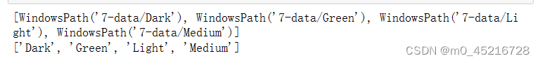
data_paths = list(data_dir.glob('*'))
print(data_paths)
# 获取类的名字
className = [str(path).split('\\')[1] for path in data_paths]

data_transforms = transforms.Compose([
    transforms.Resize([224,224]), 
    transforms.ToTensor(),
    transforms.Normalize(mean=[0.485, 0.456, 0.406], std=[0.229, 0.224, 0.225])
])

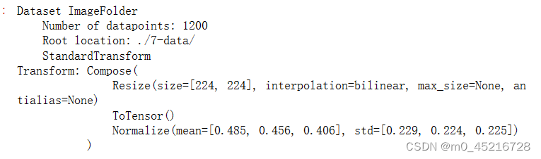
total_data = datasets.ImageFolder('./7-data/', transform=data_transforms)
total_data

1.3 划分数据

train_size = int(0.8 * len(total_data))
test_size = len(total_data) - train_size
train_dataset, test_dataset = torch.utils.data.random_split(total_data, [train_size, test_size])
# 批量
batch_size = 32
train_dl = torch.utils.data.DataLoader(train_dataset, batch_size=batch_size, shuffle = True, num_workers = 1)
test_dl = torch.utils.data.DataLoader(test_dataset, batch_size=batch_size, shuffle = True, num_workers = 1)

二、动手搭建VGG-16

13个卷积层（Convolutional Layer),分别用blockX_convX表示
5个池化层（pool layer),分别用blockX_pool表示
3个全连接层（full connected layer),分别用fcX表示VGG-16

2.1 VGG-16模型搭建

import torch.nn as nn
import torch.nn.functional as F
class vgg16(nn.Module):
    def __init__(self):
        super(vgg16,self).__init__()
        # conv1
        self.conv1 = nn.Sequential(
            nn.Conv2d(3, 64, kernel_size=(3, 3), stride=(1, 1), padding=(1, 1)),
            nn.ReLU(),
            nn.Conv2d(64, 64, kernel_size=(3, 3),stride=(1,1), padding=(1, 1)),
            nn.ReLU(),
            nn.MaxPool2d(kernel_size=(2, 2), stride=(2,2))
        )
            
        # conv2
        self.conv2 = nn.Sequential(
            nn.Conv2d(64, 128, kernel_size=(3, 3), stride=(1, 1), padding=(1, 1)),
            nn.ReLU(),
            nn.Conv2d(128, 128, kernel_size=(3, 3), stride=(1, 1), padding=(1, 1)),
            nn.ReLU(),
            nn.MaxPool2d(kernel_size=(2, 2), stride=(2, 2))
        )
        # conv3
        self.conv3 = nn.Sequential(
            nn.Conv2d(128, 256, kernel_size=(3, 3), stride=(1, 1), padding=(1, 1)),
            nn.ReLU(),
            nn.Conv2d(256, 256, kernel_size=(3, 3), stride=(1, 1), padding=(1, 1)),
            nn.ReLU(),
            nn.Conv2d(256, 256, kernel_size=(3, 3), stride=(1, 1), padding=(1, 1)),
            nn.ReLU(),
            nn.MaxPool2d(kernel_size=(2, 2), stride=(2, 2))
        )
        # conv4
        self.conv4 = nn.Sequential(
            nn.Conv2d(256, 512, kernel_size=(3, 3), stride=(1, 1), padding=(1, 1)),
            nn.ReLU(),
            nn.Conv2d(512, 512, kernel_size=(3, 3), stride=(1, 1), padding=(1, 1)),
            nn.ReLU(),
            nn.Conv2d(512, 512, kernel_size=(3, 3), stride=(1, 1), padding=(1, 1)),
            nn.ReLU(),
            nn.MaxPool2d(kernel_size=(2, 2), stride=(2, 2))
        )
         # conv5
        self.conv5 = nn.Sequential(
            nn.Conv2d(512, 512, kernel_size=(3, 3), stride=(1, 1), padding=(1, 1)),
            nn.ReLU(),
            nn.Conv2d(512, 512, kernel_size=(3, 3), stride=(1, 1), padding=(1, 1)),
            nn.ReLU(),
            nn.Conv2d(512, 512, kernel_size=(3, 3), stride=(1, 1), padding=(1, 1)),
            nn.ReLU(),
            nn.MaxPool2d(kernel_size=(2, 2), stride=(2, 2))
        )
        # fc
        self.classifier = nn.Sequential(
            nn.Linear(in_features=512*7*7, out_features=4096),
            nn.ReLU(),
            nn.Linear(in_features=4096, out_features=4096),
            nn.ReLU(),
            nn.Linear(in_features=4096, out_features=4)
        )  
    def forward(self, x):
        x = self.conv1(x)
        x = self.conv2(x)
        x = self.conv3(x)
        x = self.conv4(x)
        x = self.conv5(x)
        x = torch.flatten(x, start_dim=1)
        x = self.classifier(x)
        return x
device = 'cuda' if torch.cuda.is_available() else 'cpu'
model = vgg16().to(device)
model

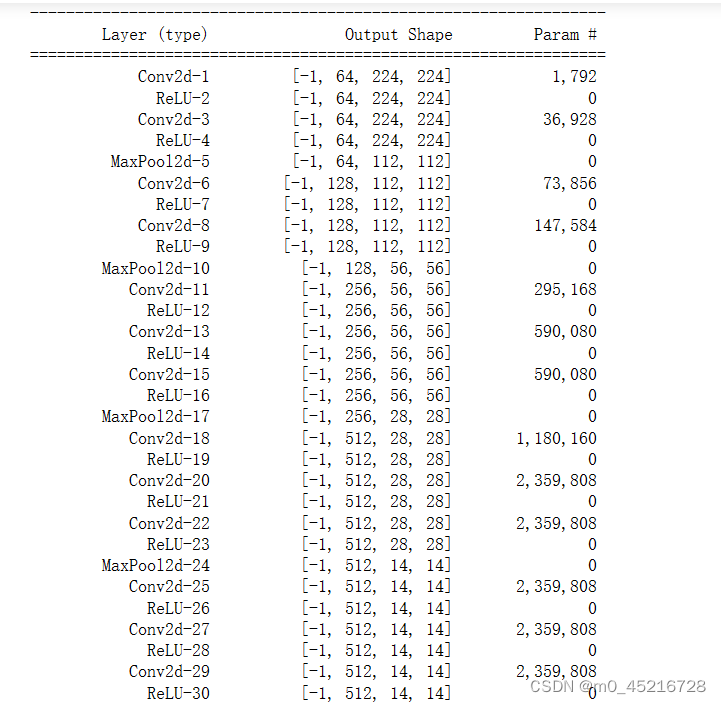
2.2 查看模型详情

import torchsummary as summary
summary.summary(model, (3, 224, 224))

三、训练模型

3.1 编写训练函数

def train(dataloader, model, loss_fun, opt):
    size = len(dataloader.dataset)
    num_batches = len(dataloader)
    train_acc, train_loss = 0, 0
    for x,y in dataloader:
        x, y = x.to(device), y.to(device)
        
        # 预测
        pred = model(x)
        loss = loss_fun(pred, y)
        
        # 反向传播
        optimizer.zero_grad()
        loss.backward()
        optimizer.step()
        
        # 记录loss与acc
        train_acc += (pred.argmax(1) == y).type(torch.float).sum().item()
        train_loss += loss.item()
    train_acc /= size
    train_loss /= num_batches
    
    return train_acc,train_loss
        

3.2 编写测试函数

def test(dataloader, model, loss_fun):
    size = len(dataloader.dataset)
    num_batches = len(dataloader)
    test_acc, test_loss = 0, 0
    with torch.no_grad():
        for x,y in dataloader:
            x, y = x.to(device), y.to(device)
            
            # 计算loss
            pred = model(x)
            loss = loss_fun(pred, y)
            
            test_loss += loss.item()
            test_acc += (pred.argmax(1)==y).type(torch.float).sum().item()
            
        test_acc /= size
        test_loss /= num_batches
    return test_acc, test_loss

3.3 正式训练

import copy
optimizer = torch.optim.Adam(model.parameters(), lr=1e-4)
loss_fun = torch.nn.CrossEntropyLoss()

epochs = 40
train_loss = []
train_acc = []
test_acc = []
test_loss = []
best_acc = 0 #设置一个最佳准确率，作为最佳模型的判别指标
for epoch in range(epochs):
    model.train()
    epoch_train_acc, epoch_train_loss = train(train_dl, model, loss_fun, optimizer)
    
    model.eval()
    epoch_test_acc, epoch_test_loss = test(test_dl, model, loss_fun)
    
    # 保存最佳模型 best_model
    if epoch_test_acc > best_acc:
        best_acc = epoch_test_acc
        best_model = copy.deepcopy(model)
        
    train_acc.append(epoch_train_acc)
    train_loss.append(epoch_train_loss)
    test_acc.append(epoch_test_acc)
    test_loss.append(epoch_test_loss)
    
    # 获取当前的学习率
    lr = optimizer.state_dict()['param_groups'][0]['lr']
    
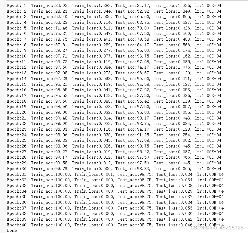
    template = ('Epoch:{:2d}, Train_acc:{:.2f}, Train_loss:{:.3f}, Test_acc:{:.2f}, Test_loss:{:.3f}, lr:{:.2E}')
    print(template.format(epoch+1, epoch_train_acc*100, epoch_train_loss, epoch_test_acc*100, epoch_test_loss, lr))

# 保存最佳模型到文件中
Path = './best_mode.pth'
torch.save(model.state_dict(), Path)

print('Done')

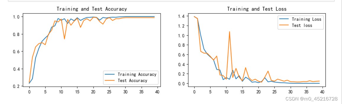
三、结果可视化

4.1 loss与Accuracy可视化

import matplotlib.pyplot as plt
plt.rcParams['font.sans-serif'] = ['SimHei']
plt.rcParams['axes.unicode_minus'] =False
plt.rcParams['figure.dpi'] = 100

plt.figure(figsize = (12,3))
plt.subplot(1,2,1)

plt.plot(range(epochs), train_acc, label='Training Accuracy')
plt.plot(range(epochs), test_acc, label='Test Accuracy')
plt.legend(loc='lower right')
plt.title('Training and Test Accuracy')

plt.subplot(1,2,2)
plt.plot(range(epochs), train_loss, label='Training Loss')
plt.plot(range(epochs), test_loss, label='Test loss')
plt.legend(loc='upper right')
plt.title('Training and Test Loss')
plt.show()

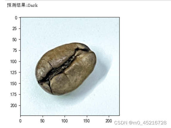
4.2 指定图片进行评估

from PIL import Image
classes = list(total_data.class_to_idx)
def pred_one_image(image_path, model, transform, classes):
    test_image = Image.open(image_path).convert('RGB')
    plt.imshow(test_image)
    
    test_image = transform(test_image)
    image = test_image.to(device).unsqueeze(0)
    
    model.eval()
    output = model(image)
    
    _,pred = torch.max(output, dim=1)
    pred_class = classes[pred]
    print('预测结果:'{pred_class})
pred_one_image(image_path='./7-data/Dark/dark(4).png',model=model, transform=train_transform, classes=classes)
 

4.3 模型评估

best_model.eval()
epoch_test_acc, epoch_test_loss = test(test_dl, best_model, loss_fun)

epoch_test_acc, epoch_test_loss

# 查看是否与记录的最高准确率一样
epoch_test_acc

将优化器改为SGD后发现惊人的现象，训练集的

import copy
optimizer = torch.optim.SGD(model.parameters(), lr=1e-4)
loss_fun = torch.nn.CrossEntropyLoss()

epochs = 40
train_loss = []
train_acc = []
test_acc = []
test_loss = []
best_acc = 0 #设置一个最佳准确率，作为最佳模型的判别指标
for epoch in range(epochs):
    model.train()
    epoch_train_acc, epoch_train_loss = train(train_dl, model, loss_fun, optimizer)
    
    model.eval()
    epoch_test_acc, epoch_test_loss = test(test_dl, model, loss_fun)
    
    # 保存最佳模型 best_model
    if epoch_test_acc > best_acc:
        best_acc = epoch_test_acc
        best_model = copy.deepcopy(model)
        
    train_acc.append(epoch_train_acc)
    train_loss.append(epoch_train_loss)
    test_acc.append(epoch_test_acc)
    test_loss.append(epoch_test_loss)
    
    # 获取当前的学习率
    lr = optimizer.state_dict()['param_groups'][0]['lr']
    
    template = ('Epoch:{:2d}, Train_acc:{:.2f}, Train_loss:{:.3f}, Test_acc:{:.2f}, Test_loss:{:.3f}, lr:{:.2E}')
    print(template.format(epoch+1, epoch_train_acc*100, epoch_train_loss, epoch_test_acc*100, epoch_test_loss, lr))

# 保存最佳模型到文件中
Path = './best_mode.pth'
torch.save(model.state_dict(), Path)

print('Done')

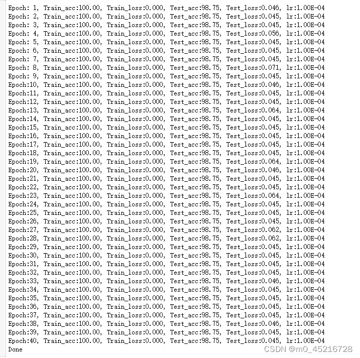
总结：

1.自己用PPT搭建网络模型，并学会如何搭建简单的卷积、池化和全连接
2.训练的速度很慢，参数量多
3.训练集和测试集在第30个epoch是能达到准确率最佳的状态
4.将优化器从Adam改为SGD后发现惊人的现象，训练集的准确率在初期就达到100%，测试集也在初期准确率就达到98.5%，并且一直维持，Adam优化器需要早30个epoch后才能达到这个效果。为什么会出现这样的情况呢？