


1.使用pytorch复现课上例题
import torch
x1, x2 = torch.Tensor([0.5]), torch.Tensor([0.3])
y1, y2 = torch.Tensor([0.23]), torch.Tensor([-0.07])
print("=====输入值:x1, x2;真实输出值:y1, y2=====")
print(x1, x2, y1, y2)
w1, w2, w3, w4, w5, w6, w7, w8 = torch.Tensor([0.2]), torch.Tensor([-0.4]), torch.Tensor([0.5]), torch.Tensor(
[0.6]), torch.Tensor([0.1]), torch.Tensor([-0.5]), torch.Tensor([-0.3]), torch.Tensor([0.8]) # 权重初始值
w1.requires_grad = True
w2.requires_grad = True
w3.requires_grad = True
w4.requires_grad = True
w5.requires_grad = True
w6.requires_grad = True
w7.requires_grad = True
w8.requires_grad = True
def sigmoid(z):
a = 1 / (1 + torch.exp(-z))
return a
def forward_propagate(x1, x2):
in_h1 = w1 * x1 + w3 * x2
out_h1 = sigmoid(in_h1) # out_h1 = torch.sigmoid(in_h1)
in_h2 = w2 * x1 + w4 * x2
out_h2 = sigmoid(in_h2) # out_h2 = torch.sigmoid(in_h2)
in_o1 = w5 * out_h1 + w7 * out_h2
out_o1 = sigmoid(in_o1) # out_o1 = torch.sigmoid(in_o1)
in_o2 = w6 * out_h1 + w8 * out_h2
out_o2 = sigmoid(in_o2) # out_o2 = torch.sigmoid(in_o2)
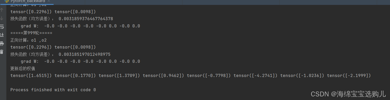
print("正向计算:o1 ,o2")
print(out_o1.data, out_o2.data)
return out_o1, out_o2
def loss_fuction(x1, x2, y1, y2): # 损失函数
y1_pred, y2_pred = forward_propagate(x1, x2) # 前向传播
loss = (1 / 2) * (y1_pred - y1) ** 2 + (1 / 2) * (y2_pred - y2) ** 2 # 考虑 : t.nn.MSELoss()
print("损失函数(均方误差):", loss.item())
return loss
def update_w(w1, w2, w3, w4, w5, w6, w7, w8):
# 步长
step = 1
w1.data = w1.data - step * w1.grad.data
w2.data = w2.data - step * w2.grad.data
w3.data = w3.data - step * w3.grad.data
w4.data = w4.data - step * w4.grad.data
w5.data = w5.data - step * w5.grad.data
w6.data = w6.data - step * w6.grad.data
w7.data = w7.data - step * w7.grad.data
w8.data = w8.data - step * w8.grad.data
w1.grad.data.zero_() # 注意:将w中所有梯度清零
w2.grad.data.zero_()
w3.grad.data.zero_()
w4.grad.data.zero_()
w5.grad.data.zero_()
w6.grad.data.zero_()
w7.grad.data.zero_()
w8.grad.data.zero_()
return w1, w2, w3, w4, w5, w6, w7, w8
if __name__ == "__main__":
print("=====更新前的权值=====")
print(w1.data, w2.data, w3.data, w4.data, w5.data, w6.data, w7.data, w8.data)
for i in range(1000):
print("=====第" + str(i) + "轮=====")
L = loss_fuction(x1, x2, y1, y2) # 前向传播,求 Loss,构建计算图
L.backward() # 自动求梯度,不需要人工编程实现。反向传播,求出计算图中所有梯度存入w中
print("\tgrad W: ", round(w1.grad.item(), 2), round(w2.grad.item(), 2), round(w3.grad.item(), 2),
round(w4.grad.item(), 2), round(w5.grad.item(), 2), round(w6.grad.item(), 2), round(w7.grad.item(), 2),
round(w8.grad.item(), 2))
w1, w2, w3, w4, w5, w6, w7, w8 = update_w(w1, w2, w3, w4, w5, w6, w7, w8)
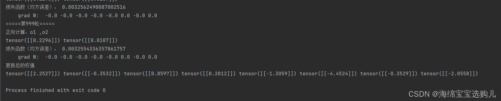
print("更新后的权值")
print(w1.data, w2.data, w3.data, w4.data, w5.data, w6.data, w7.data, w8.data)
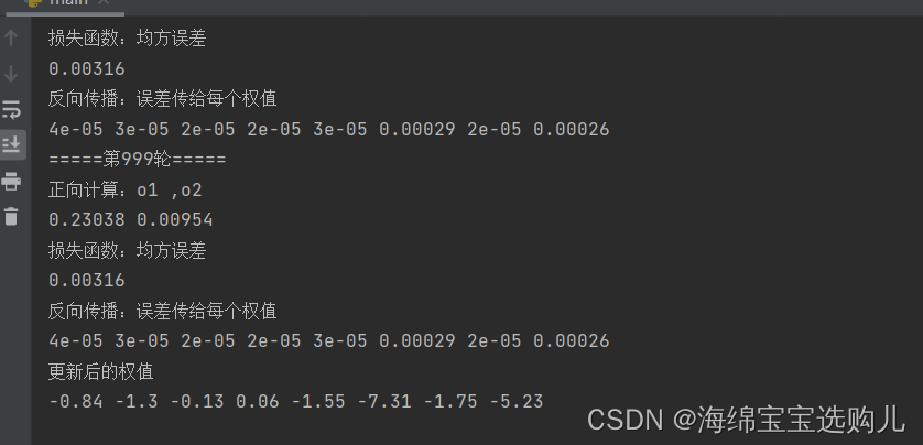
这次实现结果

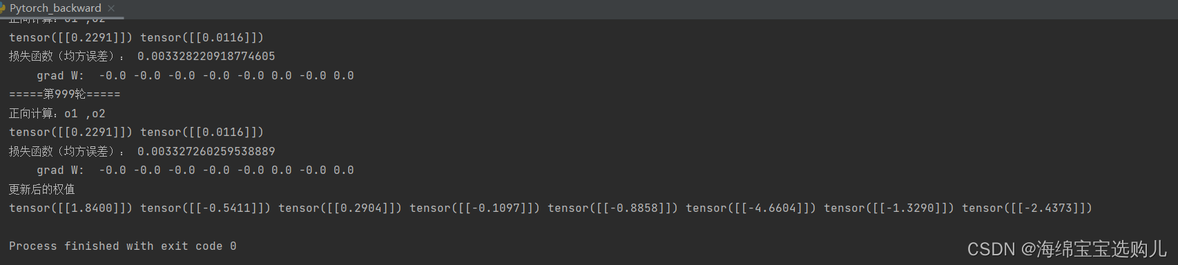
上次实验结果:
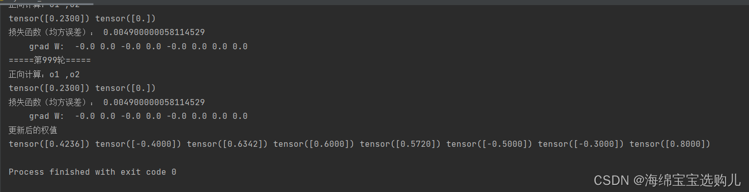
2.对比【作业3】和【作业2】的程序,观察两种方法结果是否相同?如果不同,哪个正确?
这两次的权值更新的不同,这次的程序结果是正确的。
3.【作业2】程序更新(保留【作业2中】的错误答案,留作对比。新程序到作业3。)
import numpy as np
def sigmoid(z):
a = 1 / (1 + np.exp(-z))
return a
# 前馈神经网络:
# 输入为x1,x2,输出为o1,o2,其中还有一个隐藏层为h1,h2,
# 每一层分为in操作和out操作
# in = α * a + β * b 输入流的加权累加
# out = sigmoid(in) 对加权累加的结果进行非线性变换
def forward_propagate(x1, x2, y1, y2, w1, w2, w3, w4, w5, w6, w7, w8):
in_h1 = w1 * x1 + w3 * x2 # 隐藏层
out_h1 = sigmoid(in_h1)
in_h2 = w2 * x1 + w4 * x2
out_h2 = sigmoid(in_h2)
in_o1 = w5 * out_h1 + w7 * out_h2 # out
out_o1 = sigmoid(in_o1)
in_o2 = w6 * out_h1 + w8 * out_h2
out_o2 = sigmoid(in_o2)
print("正向计算:o1 ,o2") # 输出本轮进入损失函数之前的数值out1、out2
print(round(out_o1, 5), round(out_o2, 5)) # round()舍入化整,round(x,y),y表保留小数后几位,此处保留5位小数
# 损失函数MSE 均方误差:1/n * sum((y^-y)**2)
# 此处只有2个y,所以n=2
error = (1 / 2) * (out_o1 - y1) ** 2 + (1 / 2) * (out_o2 - y2) ** 2
print("损失函数:均方误差") # 输出本轮损失函数
print(round(error, 5))
return out_o1, out_o2, out_h1, out_h2 # 返回了两层out,用于反向传播
def back_propagate(out_o1, out_o2, out_h1, out_h2):
# 反向传播
d_o1 = out_o1 - y1
d_o2 = out_o2 - y2
# print(round(d_o1, 2), round(d_o2, 2))
d_w5 = d_o1 * out_o1 * (1 - out_o1) * out_h1
d_w7 = d_o1 * out_o1 * (1 - out_o1) * out_h2
# print(round(d_w5, 2), round(d_w7, 2))
d_w6 = d_o2 * out_o2 * (1 - out_o2) * out_h1
d_w8 = d_o2 * out_o2 * (1 - out_o2) * out_h2
# print(round(d_w6, 2), round(d_w8, 2))
d_w1 = (d_o1 * out_h1 * (1 - out_h1) * w5 + d_o2 * out_o2 * (1 - out_o2) * w6) * out_h1 * (1 - out_h1) * x1
d_w3 = (d_o1 * out_h1 * (1 - out_h1) * w5 + d_o2 * out_o2 * (1 - out_o2) * w6) * out_h1 * (1 - out_h1) * x2
d_w2 = (d_o1 * out_h1 * (1 - out_h1) * w7 + d_o2 * out_o2 * (1 - out_o2) * w8) * out_h2 * (1 - out_h2) * x1
d_w4 = (d_o1 * out_h1 * (1 - out_h1) * w7 + d_o2 * out_o2 * (1 - out_o2) * w8) * out_h2 * (1 - out_h2) * x2
# print(round(d_w2, 2), round(d_w4, 2))
print("反向传播:误差传给每个权值")
print(round(d_w1, 5), round(d_w2, 5), round(d_w3, 5), round(d_w4, 5), round(d_w5, 5), round(d_w6, 5),
round(d_w7, 5), round(d_w8, 5))
return d_w1, d_w2, d_w3, d_w4, d_w5, d_w6, d_w7, d_w8
def update_w(w1, w2, w3, w4, w5, w6, w7, w8):
# 步长
step = 1
w1 = w1 - step * d_w1
w2 = w2 - step * d_w2
w3 = w3 - step * d_w3
w4 = w4 - step * d_w4
w5 = w5 - step * d_w5
w6 = w6 - step * d_w6
w7 = w7 - step * d_w7
w8 = w8 - step * d_w8
return w1, w2, w3, w4, w5, w6, w7, w8
if __name__ == "__main__":
w1, w2, w3, w4, w5, w6, w7, w8 = 0.2, -0.4, 0.5, 0.6, 0.1, -0.5, -0.3, 0.8
x1, x2 = 0.5, 0.3
y1, y2 = 0.23, -0.07
print("=====输入值:x1, x2;真实输出值:y1, y2=====")
print(x1, x2, y1, y2)
print("=====更新前的权值=====")
print(round(w1, 2), round(w2, 2), round(w3, 2), round(w4, 2), round(w5, 2), round(w6, 2), round(w7, 2),
round(w8, 2))
for i in range(1000):
print("=====第" + str(i) + "轮=====")
out_o1, out_o2, out_h1, out_h2 = forward_propagate(x1, x2, y1, y2, w1, w2, w3, w4, w5, w6, w7, w8)
d_w1, d_w2, d_w3, d_w4, d_w5, d_w6, d_w7, d_w8 = back_propagate(out_o1, out_o2, out_h1, out_h2)
w1, w2, w3, w4, w5, w6, w7, w8 = update_w(w1, w2, w3, w4, w5, w6, w7, w8)
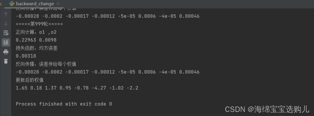
print("更新后的权值")
print(round(w1, 2), round(w2, 2), round(w3, 2), round(w4, 2), round(w5, 2), round(w6, 2), round(w7, 2),round(w8, 2))
更新后的结果,和pytorch的结果基本上相同存在一点误差。
4.对比【作业2】与【作业3】的反向传播的实现方法。总结并陈述。
错误的原因主要是慕课上的推导退错了,要正确的链式求导。具体求解过程参考以下。
5.激活函数Sigmoid用PyTorch自带函数torch.sigmoid(),观察、总结并陈述。
用torch.sigmoid()替换自己写端sigmoid函数
def forward_propagate(x1, x2):
    in_h1 = w1 * x1 + w3 * x2
    out_h1 = torch.sigmoid(in_h1)  # out_h1 = torch.sigmoid(in_h1)
    in_h2 = w2 * x1 + w4 * x2
    out_h2 = torch.sigmoid(in_h2)  # out_h2 = torch.sigmoid(in_h2)

    in_o1 = w5 * out_h1 + w7 * out_h2
    out_o1 = torch.sigmoid(in_o1)  # out_o1 = torch.sigmoid(in_o1)
    in_o2 = w6 * out_h1 + w8 * out_h2
    out_o2 = torch.sigmoid(in_o2)  # out_o2 = torch.sigmoid(in_o2)

    print("正向计算:o1 ,o2")
    print(out_o1.data, out_o2.data)

    return out_o1, out_o2
结果没啥区别。
6.激活函数Sigmoid改变为Relu,观察、总结并陈述。
def forward_propagate(x1, x2):
    in_h1 = w1 * x1 + w3 * x2
    out_h1 = torch.relu(in_h1)  # out_h1 = torch.sigmoid(in_h1)
    in_h2 = w2 * x1 + w4 * x2
    out_h2 = torch.relu(in_h2)  # out_h2 = torch.sigmoid(in_h2)

    in_o1 = w5 * out_h1 + w7 * out_h2
    out_o1 = torch.relu(in_o1)  # out_o1 = torch.sigmoid(in_o1)
    in_o2 = w6 * out_h1 + w8 * out_h2
    out_o2 = torch.relu(in_o2)  # out_o2 = torch.sigmoid(in_o2)

    print("正向计算:o1 ,o2")
    print(out_o1.data, out_o2.data)

    return out_o1, out_o2
ReLU只需要max(),计算更简单,收敛快。

7.损失函数MSE用PyTorch自带函数 t.nn.MSELoss()替代,观察、总结并陈述。
将损失函数替换为torch.nn.MSELoss()函数:
def loss_fuction(x1, x2, y1, y2):
    y1_pred, y2_pred = forward_propagate(x1, x2)
    t = torch.nn.MSELoss()
    loss = t(y1_pred,y1) + t(y2_pred,y2)
    print("损失函数(均方误差):", loss.item())
    return loss
8.损失函数MSE改变为交叉熵,观察、总结并陈述。
def loss_fuction(x1, x2, y1, y2):
    y1_pred, y2_pred = forward_propagate(x1, x2)
    loss_func = torch.nn.CrossEntropyLoss() # 创建交叉熵损失函数
    y_pred = torch.stack([y1_pred, y2_pred], dim=1)
    y = torch.stack([y1, y2], dim=1)
    loss = loss_func(y_pred, y) # 计算
    print("损失函数(均方误差):", loss.item())
    return loss

9.改变步长,训练次数,观察、总结并陈述。
step = 1
=====第999轮=====
正向计算:o1 ,o2
tensor([0.9929]) tensor([0.0072])
损失函数(均方误差): -0.018253758549690247
	grad W:  -0.0 -0.0 -0.0 -0.0 -0.0 0.0 -0.0 0.0
更新后的权值
tensor([2.2809]) tensor([0.6580]) tensor([1.7485]) tensor([1.2348]) tensor([3.8104]) tensor([-4.2013]) tensor([2.5933]) tensor([-2.0866])
step = 5
正向计算:o1 ,o2
tensor([0.9989]) tensor([0.0011])
损失函数(均方误差): -0.01962665468454361
	grad W:  -0.0 -0.0 -0.0 -0.0 -0.0 0.0 -0.0 0.0
更新后的权值
tensor([2.8660]) tensor([1.2774]) tensor([2.0996]) tensor([1.6064]) tensor([4.7890]) tensor([-5.1927]) tensor([3.3955]) tensor([-2.8994])
step = 100
=====第999轮=====
正向计算:o1 ,o2
tensor([1.0000]) tensor([4.6485e-05])
损失函数(均方误差): -0.019867710769176483
	grad W:  -0.0 -0.0 -0.0 -0.0 -0.0 0.0 -0.0 0.0
更新后的权值
tensor([3.5661]) tensor([2.0152]) tensor([2.5197]) tensor([2.0491]) tensor([6.4661]) tensor([-6.8819]) tensor([4.7917]) tensor([-4.3096])
10.权值w1-w8初始值换为随机数,对比【作业2】指定权值结果,观察、总结并陈述。
w1, w2, w3, w4, w5, w6, w7, w8 = torch.randn(1, 1), torch.randn(1, 1), torch.randn(1, 1), torch.randn(1, 1), torch.randn(1, 1), torch.randn(1, 1), torch.randn(1, 1), torch.randn(1, 1)
运行结果都有较大差别说明权值的选择也很重要。
11.全面总结反向传播原理和编码实现,认真写心得体会。
反向传播原理:通过反向传播不断的优化权值来优化模型使损失函数最小。我们这次作业更深入的理解了神经网络,学会了反向传播的具体实现(链式法则),也练习了python的使用有较大的提升。


 1420
1420


 被折叠的 条评论
为什么被折叠?
被折叠的 条评论
为什么被折叠?
 到【灌水乐园】发言


