


本代码最初在colab中实现,以下为全部代码及运行输出结果
1.挂载谷歌云盘,解压数据集
%pwd
‘/content’
!unzip '/content/drive/MyDrive/AI_content/RCNN/Images.zip' -d '/content/drive/MyDrive/AI_content/RCNN'
!unzip '/content/drive/MyDrive/AI_content/RCNN/Airplanes_Annotations.zip' -d '/content/drive/MyDrive/AI_content/RCNN'
2.安装并导入依赖
!pip install tensorflow==2.8.0
import os,cv2,keras
import pandas as pd
import matplotlib.pyplot as plt
import numpy as np
import tensorflow as tf
tf.__version__
‘2.8.0’
3.更改工作目录
cd /content/drive/MyDrive/AI_content/RCNN
/content/drive/MyDrive/AI_content/RCNN
path = '/content/drive/MyDrive/AI_content/RCNN/Images'
annot = '/content/drive/MyDrive/AI_content/RCNN/Airplanes_Annotations'
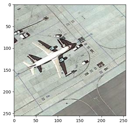
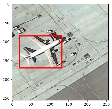
4.查看数据和标签
Index=148
filename = "airplane_"+str(Index)+".jpg"
print(filename)
img = cv2.imread(os.path.join(path,filename))
df = pd.read_csv(os.path.join(annot,filename.replace(".jpg",".csv")))
plt.imshow(img)
for row in df.iterrows():
    x1 = int(row[1][0].split(" ")[0])
    y1 = int(row[1][0].split(" ")[1])
    x2 = int(row[1][0].split(" ")[2])
    y2 = int(row[1][0].split(" ")[3])
    cv2.rectangle(img,(x1,y1),(x2,y2),(255,0,0), 2)

plt.figure()
plt.imshow(img)
plt.show()
airplane_148.jpg
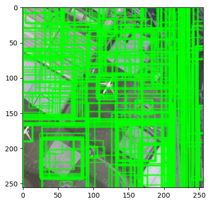
5.Selective search
cv2.setUseOptimized(True);
ss = cv2.ximgproc.segmentation.createSelectiveSearchSegmentation()
im = cv2.imread(os.path.join(path,"42850.jpg"))
ss.setBaseImage(im)
ss.switchToSelectiveSearchFast()
rects = ss.process()
imOut = im.copy() #复制原图,在复制后的图片上绘制矩形
for i, rect in (enumerate(rects)):
    x, y, w, h = rect
    cv2.rectangle(imOut, (x, y), (x+w, y+h), (0, 255, 0), 1, cv2.LINE_AA) #在imOut上绘制矩形

plt.imshow(imOut)

# 显示可视化的结果
plt.show()
6.IOU
def get_iou(bb1, bb2):
  # assuring for proper dimension.
    assert bb1['x1'] < bb1['x2']
    assert bb1['y1'] < bb1['y2']
    assert bb2['x1'] < bb2['x2']
    assert bb2['y1'] < bb2['y2']
  # calculating dimension of common area between these two boxes.
    x_left = max(bb1['x1'], bb2['x1'])
    y_top = max(bb1['y1'], bb2['y1'])
    x_right = min(bb1['x2'], bb2['x2'])
    y_bottom = min(bb1['y2'], bb2['y2'])
  # if there is no overlap output 0 as intersection area is zero.
    if x_right < x_left or y_bottom < y_top:
        return 0.0
  # calculating intersection area.
    intersection_area = (x_right - x_left) * (y_bottom - y_top)
  # individual areas of both these bounding boxes.
    bb1_area = (bb1['x2'] - bb1['x1']) * (bb1['y2'] - bb1['y1'])
    bb2_area = (bb2['x2'] - bb2['x1']) * (bb2['y2'] - bb2['y1'])
  # union area = area of bb1_+ area of bb2 - intersection of bb1 and bb2.
    iou = intersection_area / float(bb1_area + bb2_area - intersection_area)
    assert iou >= 0.0
    assert iou <= 1.0
    return iou
7.准备训练数据
# At the end of below code we will have our train data in these lists
train_images=[]
train_labels=[]
for e,i in enumerate(os.listdir(annot)):
    try:
        if i.startswith("airplane"):
            filename = i.split(".")[0]+".jpg"
            print(e,filename)
            # 读取图像
            image = cv2.imread(os.path.join(path,filename))
            # 读取标注文件
            df = pd.read_csv(os.path.join(annot,i))
            gtvalues=[]
            for row in df.iterrows():
                x1 = int(row[1][0].split(" ")[0])
                y1 = int(row[1][0].split(" ")[1])
                x2 = int(row[1][0].split(" ")[2])
                y2 = int(row[1][0].split(" ")[3])
                gtvalues.append({"x1":x1,"x2":x2,"y1":y1,"y2":y2})
            # 设置基础图像
            ss.setBaseImage(image)   # setting given image as base image
            ss.switchToSelectiveSearchFast()     # running selective search on base image

            # 运行选择性搜索
            ssresults = ss.process()     # processing to get the outputs
            imout = image.copy()
            counter = 0
            falsecounter = 0
            flag = 0
            fflag = 0
            bflag = 0
             # 遍历选择性搜索的结果
            for e,result in enumerate(ssresults):
                if e < 2000 and flag == 0:     # till 2000 to get top 2000 regions only
                    for gtval in gtvalues:
                        x,y,w,h = result
                        iou = get_iou(gtval,{"x1":x,"x2":x+w,"y1":y,"y2":y+h})  # calculating IoU for each of the proposed regions
                        if counter < 30:       # getting only 30 psoitive examples
                            if iou > 0.70:     # IoU of being positive is 0.7
                                timage = imout[x:x+w,y:y+h]
                                resized = cv2.resize(timage, (224,224), interpolation = cv2.INTER_AREA)
                                train_images.append(resized)
                                train_labels.append(1)
                                counter += 1
                        else :
                            fflag =1              # to insure we have collected all psotive examples
                        if falsecounter <30:      # 30 negatve examples are allowed only
                            if iou < 0.3:         # IoU of being negative is 0.3
                                timage = imout[x:x+w,y:y+h]
                                resized = cv2.resize(timage, (224,224), interpolation = cv2.INTER_AREA)
                                train_images.append(resized)
                                train_labels.append(0)
                                falsecounter += 1
                        else :
                            bflag = 1             #to ensure we have collected all negative examples
                    if fflag == 1 and bflag == 1:
                        print("inside")
                        flag = 1        # to signal the complition of data extaction from a particular image
    except Exception as e:
        print(e)
        print("error in "+filename)
        continue
# conversion of train data into arrays for further training
X_new = np.array(train_images)
Y_new = np.array(train_labels)
# 为方便下次不用重新处理输入的训练数据,在这里将X_new,Y_new进行保存
np.save('save_X_new',X_new)
np.save('save_Y_new',Y_new)
# 读取保存的数据X_new,Y_new
X_new = np.load('save_X_new.npy')
Y_new = np.load('save_Y_new.npy')
# 这里因为colab提供的显存不够,只有15g,加载全部数据进去会爆显存,所以只截取一部分样本来进行训练,即X_new_subset 、Y_new_subset
total_nums = len(Y_new)
print(total_nums)
30229
# 从训练数据中随机选择 10000 个样本
num_samples = 5000
random_indices = np.random.choice(len(X_new), num_samples, replace=False)

# 使用随机选择的索引来获取样本
X_new_subset = X_new[random_indices]
Y_new_subset = Y_new[random_indices]
8.预训练(使用VGG16模型创建一个迁移学习模型)
from keras.layers import Dense
from keras import Model
from keras import optimizers
# 使用 VGG16 模型来创建一个迁移学习模型
vgg = tf.keras.applications.vgg16.VGG16(include_top=True, weights='imagenet', input_tensor=None, input_shape=None, pooling=None, classes=1000)
# 将 VGG16 模型的大部分层设为不可训练,保留最后两层的可训练性
for layer in vgg.layers[:-2]:
  layer.trainable = False
# 获取 VGG16 模型中名为 'fc2' 的层,并获取该层的输出
x = vgg.get_layer('fc2')
last_output =  x.output
# 在 VGG16 模型的 'fc2' 层之后添加了一个新的全连接层,这个全连接层只有一个单元,使用 sigmoid 激活函数来输出二元分类的概率
x = tf.keras.layers.Dense(1,activation = 'sigmoid')(last_output)
# 创建一个新的模型,该模型接受 VGG16 的输入,并输出通过添加新层后的结果
model = tf.keras.Model(vgg.input,x)
# 编译模型,使用 Adam 优化器,二元交叉熵作为损失函数进行训练,并监控模型的精度(accuracy)指标
model.compile(optimizer = "adam",
              loss = 'binary_crossentropy',
              metrics = ['acc'])
# 保存一下这个模型文件
model.save('my_model_vgg16.h5')
/usr/local/lib/python3.10/dist-packages/keras/src/engine/training.py:3103: UserWarning: You are saving your model as an HDF5 file via
model.save(). This file format is considered legacy. We recommend using instead the native Keras format, e.g.model.save('my_model.keras'). saving_api.save_model(
# 查看模型结构并进行训练
model.summary()
model.fit(X_new_subset,Y_new_subset,batch_size = 32,epochs = 3, verbose = 1,validation_split=.05,shuffle = True)
Model: "model"
_________________________________________________________________
 Layer (type)                Output Shape              Param #
=================================================================
 input_1 (InputLayer)        [(None, 224, 224, 3)]     0

 block1_conv1 (Conv2D)       (None, 224, 224, 64)      1792

 block1_conv2 (Conv2D)       (None, 224, 224, 64)      36928

 block1_pool (MaxPooling2D)  (None, 112, 112, 64)      0

 block2_conv1 (Conv2D)       (None, 112, 112, 128)     73856

 block2_conv2 (Conv2D)       (None, 112, 112, 128)     147584

 block2_pool (MaxPooling2D)  (None, 56, 56, 128)       0

 block3_conv1 (Conv2D)       (None, 56, 56, 256)       295168

 block3_conv2 (Conv2D)       (None, 56, 56, 256)       590080

 block3_conv3 (Conv2D)       (None, 56, 56, 256)       590080

 block3_pool (MaxPooling2D)  (None, 28, 28, 256)       0

 block4_conv1 (Conv2D)       (None, 28, 28, 512)       1180160

 block4_conv2 (Conv2D)       (None, 28, 28, 512)       2359808

 block4_conv3 (Conv2D)       (None, 28, 28, 512)       2359808

 block4_pool (MaxPooling2D)  (None, 14, 14, 512)       0

 block5_conv1 (Conv2D)       (None, 14, 14, 512)       2359808

 block5_conv2 (Conv2D)       (None, 14, 14, 512)       2359808

 block5_conv3 (Conv2D)       (None, 14, 14, 512)       2359808

 block5_pool (MaxPooling2D)  (None, 7, 7, 512)         0

 flatten (Flatten)           (None, 25088)             0

 fc1 (Dense)                 (None, 4096)              102764544

 fc2 (Dense)                 (None, 4096)              16781312

 dense (Dense)               (None, 1)                 4097

=================================================================
Total params: 134264641 (512.18 MB)
Trainable params: 16785409 (64.03 MB)
Non-trainable params: 117479232 (448.15 MB)
_________________________________________________________________
Epoch 1/3
149/149 [==============================] - 43s 214ms/step - loss: 1.4586 - acc: 0.7680 - val_loss: 0.3230 - val_acc: 0.8880
Epoch 2/3
149/149 [==============================] - 19s 129ms/step - loss: 0.3880 - acc: 0.8215 - val_loss: 0.3339 - val_acc: 0.8560
Epoch 3/3
149/149 [==============================] - 20s 131ms/step - loss: 0.3464 - acc: 0.8495 - val_loss: 0.3104 - val_acc: 0.8760

<keras.src.callbacks.History at 0x7a67e60b2140>
9.创建带有SVM的新网络
9.1创建供SVM使用的数据集
svm_image = [];
svm_label = [];
# 创建SVM数据集采用了和训练数据集不同的iou标准
for e,i in enumerate(os.listdir(annot)):
    try:
        if i.startswith("airplane"):
            # 提取图像文件名并读取图像
            filename = i.split(".")[0]+".jpg"
            print(e,filename)
            image = cv2.imread(os.path.join(path,filename))

            # 读取对应的标注文件
            df = pd.read_csv(os.path.join(annot,i))
            gtvalues=[]

            # 解析标注文件中的目标坐标信息
            for row in df.iterrows():
                x1 = int(row[1][0].split(" ")[0])
                y1 = int(row[1][0].split(" ")[1])
                x2 = int(row[1][0].split(" ")[2])
                y2 = int(row[1][0].split(" ")[3])
                gtvalues.append({"x1":x1,"x2":x2,"y1":y1,"y2":y2})

                # 从图像中截取目标区域并调整大小,作为正样本(ground_truth对应的图像区域,作为正样本)
                timage = image[x1:x2,y1:y2]
                resized = cv2.resize(timage, (224,224), interpolation = cv2.INTER_AREA)
                svm_image.append(resized)
                svm_label.append([0,1])# 正样本标签 [0, 1]

            # 执行选择性搜索算法获取区域建议
            ss.setBaseImage(image)
            ss.switchToSelectiveSearchFast()
            ssresults = ss.process()
            imout = image.copy()
            counter = 0
            falsecounter = 0
            flag = 0

             # 遍历选择性搜索结果以构建负样本
            for e,result in enumerate(ssresults):
                if e < 2000 and flag == 0:
                    for gtval in gtvalues:
                        x,y,w,h = result
                        iou = get_iou(gtval,{"x1":x,"x2":x+w,"y1":y,"y2":y+h})

                        # 添加满足条件的负样本
                        if falsecounter <5:
                            if iou < 0.3:
                                timage = imout[x:x+w,y:y+h]
                                resized = cv2.resize(timage, (224,224), interpolation = cv2.INTER_AREA)
                                svm_image.append(resized)
                                svm_label.append([1,0]) # 负样本标签 [1, 0]
                                falsecounter += 1
                        else :
                            flag = 1 # 达到负样本数量上限
    except Exception as e:
        print(e)
        print("error in "+filename)
        continue
# 为防止RAM不够,这里把svm_image、svm_label也只选取一部分
X_svm = np.array(svm_image)
Y_svm = np.array(svm_label)
# 为方便下次不用重新处理输入的训练数据,在这里将X_new,Y_new进行保存
np.save('save_X_svm',X_svm)
np.save('save_Y_svm',Y_svm)
total_nums_svm = len(Y_svm)
print(total_nums_svm)
7750
X_svm = np.load('save_X_svm.npy')
Y_svm = np.load('save_Y_svm.npy')
# 从训练数据中随机选择 2000 个样本
num_samples = 2000
random_indices = np.random.choice(len(X_svm), num_samples, replace=False)

# 使用随机选择的索引来获取样本
X_svm_subset = X_svm[random_indices]
Y_svm_subset = Y_svm[random_indices]
9.2 SVM模型结构
# 从现有模型中获取 'fc2' 层的输出
x = model.get_layer('fc2').output

# 添加一个具有2个单元的全连接层,没有激活函数
Y = tf.keras.layers.Dense(2)(x)

# 创建一个新的模型,该模型接收现有模型的输入,并输出新添加的全连接层的结果
final_model = tf.keras.Model(model.input, Y)

# 编译新模型
final_model.compile(loss='hinge',  # 使用hinge loss损失函数
                    optimizer='adam',  # 优化器为 Adam
                    metrics=['accuracy'])  # 监控模型的准确度指标

# 输出新模型的概要信息
final_model.summary()

# 加载预训练模型的权重
# final_model.load_weights('my_model_weights.h5')
Model: "model_1"
_________________________________________________________________
 Layer (type)                Output Shape              Param #
=================================================================
 input_1 (InputLayer)        [(None, 224, 224, 3)]     0

 block1_conv1 (Conv2D)       (None, 224, 224, 64)      1792

 block1_conv2 (Conv2D)       (None, 224, 224, 64)      36928

 block1_pool (MaxPooling2D)  (None, 112, 112, 64)      0

 block2_conv1 (Conv2D)       (None, 112, 112, 128)     73856

 block2_conv2 (Conv2D)       (None, 112, 112, 128)     147584

 block2_pool (MaxPooling2D)  (None, 56, 56, 128)       0

 block3_conv1 (Conv2D)       (None, 56, 56, 256)       295168

 block3_conv2 (Conv2D)       (None, 56, 56, 256)       590080

 block3_conv3 (Conv2D)       (None, 56, 56, 256)       590080

 block3_pool (MaxPooling2D)  (None, 28, 28, 256)       0

 block4_conv1 (Conv2D)       (None, 28, 28, 512)       1180160

 block4_conv2 (Conv2D)       (None, 28, 28, 512)       2359808

 block4_conv3 (Conv2D)       (None, 28, 28, 512)       2359808

 block4_pool (MaxPooling2D)  (None, 14, 14, 512)       0

 block5_conv1 (Conv2D)       (None, 14, 14, 512)       2359808

 block5_conv2 (Conv2D)       (None, 14, 14, 512)       2359808

 block5_conv3 (Conv2D)       (None, 14, 14, 512)       2359808

 block5_pool (MaxPooling2D)  (None, 7, 7, 512)         0

 flatten (Flatten)           (None, 25088)             0

 fc1 (Dense)                 (None, 4096)              102764544

 fc2 (Dense)                 (None, 4096)              16781312

 dense_1 (Dense)             (None, 2)                 8194

=================================================================
Total params: 134268738 (512.19 MB)
Trainable params: 16789506 (64.05 MB)
Non-trainable params: 117479232 (448.15 MB)
_________________________________________________________________
9.3 模型训练
# 使用 SVM 数据集对最终模型进行训练,训练过程中的结果将存储在 hist_final 中
hist_final = final_model.fit(
    X_svm_subset,  # SVM 数据集中的图像数据
    Y_svm_subset,  # SVM 数据集中的标签数据
    batch_size=32,        # 批处理大小
    epochs=20,            # 迭代次数
    verbose=1,            # 训练过程中输出日志的详细程度(1为详细输出,0为不输出)
    shuffle=True,         # 在每个 epoch 开始时是否对数据进行洗牌
    validation_split=0.05  # 验证集的拆分比例,这里设置为 0.05 表示将 5% 的数据作为验证集
)
Epoch 1/20
60/60 [==============================] - 17s 217ms/step - loss: 0.7543 - accuracy: 0.6689 - val_loss: 0.7870 - val_accuracy: 0.6100
Epoch 2/20
60/60 [==============================] - 8s 128ms/step - loss: 0.5756 - accuracy: 0.7463 - val_loss: 0.6612 - val_accuracy: 0.7200
Epoch 3/20
60/60 [==============================] - 8s 134ms/step - loss: 0.4762 - accuracy: 0.7905 - val_loss: 0.6471 - val_accuracy: 0.7300
Epoch 4/20
60/60 [==============================] - 8s 132ms/step - loss: 0.4303 - accuracy: 0.8232 - val_loss: 0.7102 - val_accuracy: 0.6900
Epoch 5/20
60/60 [==============================] - 8s 131ms/step - loss: 0.4178 - accuracy: 0.8200 - val_loss: 0.6434 - val_accuracy: 0.7000
Epoch 6/20
60/60 [==============================] - 8s 136ms/step - loss: 0.3378 - accuracy: 0.8558 - val_loss: 0.7106 - val_accuracy: 0.7000
Epoch 7/20
60/60 [==============================] - 8s 135ms/step - loss: 0.3321 - accuracy: 0.8647 - val_loss: 0.6975 - val_accuracy: 0.7400
Epoch 8/20
60/60 [==============================] - 8s 130ms/step - loss: 0.3007 - accuracy: 0.8737 - val_loss: 0.7403 - val_accuracy: 0.7500
Epoch 9/20
60/60 [==============================] - 8s 138ms/step - loss: 0.2735 - accuracy: 0.8858 - val_loss: 0.8128 - val_accuracy: 0.7100
Epoch 10/20
60/60 [==============================] - 8s 133ms/step - loss: 0.2241 - accuracy: 0.9153 - val_loss: 0.9183 - val_accuracy: 0.6900
Epoch 11/20
60/60 [==============================] - 8s 141ms/step - loss: 0.2732 - accuracy: 0.8916 - val_loss: 0.7814 - val_accuracy: 0.7100
Epoch 12/20
60/60 [==============================] - 8s 142ms/step - loss: 0.2009 - accuracy: 0.9163 - val_loss: 0.8467 - val_accuracy: 0.7100
Epoch 13/20
60/60 [==============================] - 8s 140ms/step - loss: 0.2214 - accuracy: 0.9126 - val_loss: 0.7389 - val_accuracy: 0.7500
Epoch 14/20
60/60 [==============================] - 9s 144ms/step - loss: 0.1761 - accuracy: 0.9268 - val_loss: 0.8726 - val_accuracy: 0.7300
Epoch 15/20
60/60 [==============================] - 9s 142ms/step - loss: 0.1645 - accuracy: 0.9295 - val_loss: 0.7956 - val_accuracy: 0.7400
Epoch 16/20
60/60 [==============================] - 9s 142ms/step - loss: 0.1385 - accuracy: 0.9453 - val_loss: 0.7979 - val_accuracy: 0.7200
Epoch 17/20
60/60 [==============================] - 8s 138ms/step - loss: 0.1303 - accuracy: 0.9495 - val_loss: 0.8370 - val_accuracy: 0.7700
Epoch 18/20
60/60 [==============================] - 8s 139ms/step - loss: 0.1469 - accuracy: 0.9426 - val_loss: 0.7578 - val_accuracy: 0.7900
Epoch 19/20
60/60 [==============================] - 9s 143ms/step - loss: 0.1020 - accuracy: 0.9611 - val_loss: 0.7946 - val_accuracy: 0.7600
Epoch 20/20
60/60 [==============================] - 9s 147ms/step - loss: 0.1020 - accuracy: 0.9632 - val_loss: 0.8619 - val_accuracy: 0.7500
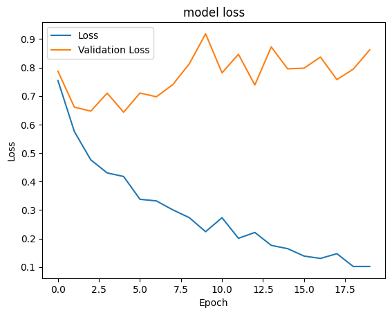
9.4 绘制损失变化曲线
# 绘制模型训练过程中的损失变化曲线
plt.plot(hist_final.history['loss'])        # 训练集的损失
plt.plot(hist_final.history['val_loss'])    # 验证集的损失
plt.title("model loss")                     # 图像标题
plt.ylabel("Loss")                          # y 轴标签为损失
plt.xlabel("Epoch")                         # x 轴标签为 epoch
plt.legend(["Loss", "Validation Loss"])     # 添加图例,分别对应训练集和验证集的损失
plt.show()                                  # 显示图像

plt.savefig('chart_loss.png')               # 保存图像为文件(在 plt.show() 之后保存是无效的,应该放在 plt.show() 之前)
10. 测试
###########  it's time for test a image    ##########
image = cv2.imread(os.path.join(path,'airplane_020.jpg'))


ss.setBaseImage(image) # 设置选择性搜索算法的基础图像为读取的图像
ss.switchToSelectiveSearchFast() # 使用选择性搜索算法的快速模式
ssresults = ss.process() # 对基础图像执行选择性搜索,获取区域建议

imOut = image.copy() # 创建图像的副本,用于绘制矩形框
boxes = [] # 存储被判断为飞机区域的边界框信息
count = 0 # 计数器:记录被判断为飞机区域的数量

# 对选择性搜索结果的前 50 个区域建议进行处理
for e,result in enumerate(ssresults):
  if e < 50:
    x,y,w,h = result

    timage = imout[x:x+w,y:y+h] # 从原始图像中获取当前建议区域的图像部分
    resized = cv2.resize(timage, (224,224), interpolation = cv2.INTER_AREA) # 调整图像大小为模型的输入尺寸
    resized = np.expand_dims(resized,axis = 0) # 将图像扩展一个维度以适应模型输入的要求
    out = final_model.predict(resized)  # 使用最终的模型对该区域进行预测,得到输出结果
    print(e,out)

    if(out[0][0]<out[0][1]): # 如果模型判断该区域可能包含飞机
      boxes.append([x,y,w,h]) # 将边界框信息添加到列表中,并增加计数器
      count+=1

# 对被判断为飞机区域的边界框进行处理
for box in boxes:
    x, y, w, h = box
    print(x,y,w,h)
#     imOut = imOut[x:x+w,y:y+h]
    # 在原始图像上绘制矩形框,以突出显示这些被判断为飞机的区域
    cv2.rectangle(imOut, (x, y), (x+w, y+h), (0, 255, 0), 1, cv2.LINE_AA)

plt.imshow(imOut)
plt.show()
1/1 [==============================] - 1s 1s/step
0 [[ 2.551831  -2.6361141]]
1/1 [==============================] - 0s 31ms/step
1 [[ 1.2116516 -1.1462703]]
1/1 [==============================] - 0s 43ms/step
2 [[ 3.1247723 -3.0577419]]
1/1 [==============================] - 0s 38ms/step
3 [[ 0.3094477  -0.35184118]]
1/1 [==============================] - 0s 33ms/step
4 [[ 16.334412 -16.097301]]
1/1 [==============================] - 0s 36ms/step
5 [[-1.9055386  1.8246138]]
1/1 [==============================] - 0s 46ms/step
6 [[ 3.849068 -3.596069]]
1/1 [==============================] - 0s 35ms/step
7 [[-4.3343387  4.457566 ]]
1/1 [==============================] - 0s 28ms/step
8 [[ 2.1157243 -2.0935826]]
1/1 [==============================] - 0s 37ms/step
9 [[ 1.1227907 -1.0547544]]
1/1 [==============================] - 0s 32ms/step
10 [[ 3.028215  -3.0655315]]
1/1 [==============================] - 0s 35ms/step
11 [[-3.4406524  3.4818974]]
1/1 [==============================] - 0s 36ms/step
12 [[-3.3148727  3.2502732]]
1/1 [==============================] - 0s 69ms/step
13 [[-1.7705667  1.8401496]]
1/1 [==============================] - 0s 119ms/step
14 [[ 17.1168   -17.020542]]
1/1 [==============================] - 0s 31ms/step
15 [[-0.54532474  0.49859324]]
1/1 [==============================] - 0s 39ms/step
16 [[ 1.3955598 -1.4487445]]
1/1 [==============================] - 0s 39ms/step
17 [[-0.9255678  0.7681236]]
1/1 [==============================] - 0s 34ms/step
18 [[-1.0967708  1.0601681]]
1/1 [==============================] - 0s 35ms/step
19 [[ 1.6157322 -1.5883387]]
1/1 [==============================] - 0s 19ms/step
20 [[ 6.222667 -6.078978]]
1/1 [==============================] - 0s 22ms/step
21 [[ 1.9781907 -1.9643315]]
1/1 [==============================] - 0s 21ms/step
22 [[ 2.6352754 -2.6751401]]
1/1 [==============================] - 0s 22ms/step
23 [[-0.6199166  0.6234232]]
1/1 [==============================] - 0s 26ms/step
24 [[ 0.56931984 -0.52301127]]
1/1 [==============================] - 0s 19ms/step
25 [[-4.092036   4.0529504]]
1/1 [==============================] - 0s 20ms/step
26 [[-1.1211745  1.1134607]]
1/1 [==============================] - 0s 20ms/step
27 [[ 1.5422791 -1.504165 ]]
1/1 [==============================] - 0s 20ms/step
28 [[ 0.9709082 -1.1293985]]
1/1 [==============================] - 0s 22ms/step
29 [[ 6.2005806 -6.223065 ]]
1/1 [==============================] - 0s 19ms/step
30 [[ 0.7283702  -0.67930716]]
1/1 [==============================] - 0s 20ms/step
31 [[ 3.7712991 -3.7369084]]
1/1 [==============================] - 0s 20ms/step
32 [[ 1.7139057 -1.7024881]]
1/1 [==============================] - 0s 21ms/step
33 [[ 12.521779 -12.554838]]
1/1 [==============================] - 0s 24ms/step
34 [[ 3.4832761 -3.3890066]]
1/1 [==============================] - 0s 23ms/step
35 [[ 1.2881904 -1.3030462]]
1/1 [==============================] - 0s 31ms/step
36 [[ 1.3349662 -1.2856408]]
1/1 [==============================] - 0s 20ms/step
37 [[ 0.29870683 -0.25320527]]
1/1 [==============================] - 0s 20ms/step
38 [[-1.2835077  1.3210849]]
1/1 [==============================] - 0s 19ms/step
39 [[ 1.3556112 -1.3576012]]
1/1 [==============================] - 0s 20ms/step
40 [[ 5.945995  -5.7617545]]
1/1 [==============================] - 0s 20ms/step
41 [[ 4.5127177 -4.54366  ]]
1/1 [==============================] - 0s 19ms/step
42 [[ 1.2226268 -1.2334687]]
1/1 [==============================] - 0s 19ms/step
43 [[ 2.2175348 -2.1676831]]
1/1 [==============================] - 0s 20ms/step
44 [[ 5.3103013 -5.1500263]]
1/1 [==============================] - 0s 22ms/step
45 [[ 1.7600315 -1.8218967]]
1/1 [==============================] - 0s 20ms/step
46 [[ 3.2599857 -2.9830909]]
1/1 [==============================] - 0s 19ms/step
47 [[-1.2734337  1.2411362]]
1/1 [==============================] - 0s 21ms/step
48 [[ 10.405064 -10.193722]]
1/1 [==============================] - 0s 20ms/step
49 [[-1.247491   1.2709295]]
145 129 35 31
0 71 98 70
176 148 64 43
49 91 49 22
0 71 77 70
199 148 38 29
174 130 21 27
19 95 58 45
111 142 27 23
120 127 32 33
0 74 48 53
120 143 33 19
29 149 36 40
111 117 34 46
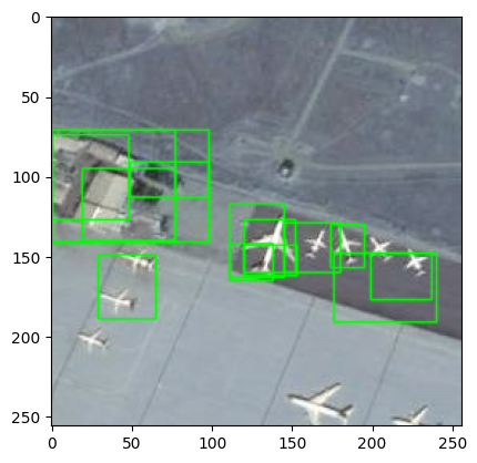
最后的测试效果没有很好,可能因为使用的训练数据过少,如果显存足够可以不用截取训练集的子集来进行训练,效果应该会提高。


 600
600


 被折叠的 条评论
为什么被折叠?
被折叠的 条评论
为什么被折叠?
 到【灌水乐园】发言


