4D NeRF 场景重建方法总结

Neural 3D Video

Paper: Li T, Slavcheva M, Zollhoefer M, et al. Neural 3d video synthesis from multi-view video[C]//Proceedings of the IEEE/CVF Conference on Computer Vision and Pattern Recognition. 2022: 5521-5531.
Introduction: https://neural-3d-video.github.io/
Code: https://github.com/facebookresearch/Neural_3D_Video

Neural 3D Video 是一种动态 NeRF 表示方法，使用一组紧凑的时间隐变量将 NeRF 扩展到时间维度，然后通过分层抽样和重要性采样实现 4D 场景的快速渲染。此外，作者还采集了 DyNeRF 数据集，广泛为后续研究所用。

一. 4D Representation

为了处理 4D 场景，需要在 NeRF 的 MLP 上添加输入变量 $t$，但这在处理拓扑变化等复杂场景时效果较差。因此，Neural 3D Video 学习一个与时间相关的隐变量 $z_t$ 来紧凑表示动态场景的时间变量：
$$F_{\Theta }:\left(\mathbf{x},\mathbf{d},{\mathbf{z}}_t\right)⟶(\mathbf{c},\sigma )$$

在训练开始前，所有的 ${\mathbf{z}}_t$ 被随机初始化。训练过程中联合优化 4D 网络参数和时间隐变量。渲染过程同 NeRF：
$$\begin{array}{rl}{\mathbf{C}}^{(t)}(\mathbf{r})& ={\int }_{s_n}^{s_f}T(s)\sigma \left(\mathbf{r}(s),{\mathbf{z}}_t\right)\mathbf{c}\left(\mathbf{r}(s),\mathbf{d},{\mathbf{z}}_t\right)ds,\\ & \text{where }T(s)=\exp \left(-{\int }_{s_n}^s\sigma \left(\mathbf{r}(p),{\mathbf{z}}_t\right)\right)dp)\end{array}$$

二. Efficient Training

因为一组 4D 同步视频存在大量的时间不变量和冗余，所以需要更加紧凑的 4D 表示方法。Neural 3D Video 采用以下两个策略加速训练：

1. Hierarchical Training：先按照一定间隔采样关键帧进行训练，然后再对中间帧进行插值比较损失；
2. Ray Importance Sampling：在关键帧和非关键帧的训练中，都对光线进行重要性采样，即采样随时间变化较大的像素点进行训练；

总的损失函数如下：
L efficient  = ∑ t ∈ S , r ∈ I ∑ j ∈ { c , f } ∥ C ^ j ( t ) ( r ) − C ( t ) ( r ) ∥ 2 2 \mathcal{L}_{\text {efficient }}=\sum_{t \in \mathcal{S}, \mathbf{r} \in \mathcal{I}} \sum_{j \in\{c, f\}}\left\|\hat{\mathbf{C}}_j^{(t)}(\mathbf{r})-\mathbf{C}^{(t)}(\mathbf{r})\right\|_2^2 Lefficient ​=t∈S,r∈I∑​j∈{c,f}∑​ ​C^j(t)​(r)−C(t)(r) ​22​

Nerfies

Hypernerf

Paper: Park K, Sinha U, Hedman P, et al. Hypernerf: A higher-dimensional representation for topologically varying neural radiance fields[J]. arXiv preprint arXiv:2106.13228, 2021.
Introduction: https://hypernerf.github.io/
Code: https://github.com/google/hypernerf

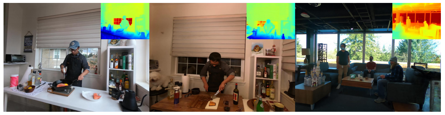
Hypernerf 是 Nerfies 的作者 Keunhong Park 等人鉴于 Nerfies 无法建模拓扑变化进一步改进得到的动态 NeRF 表示方法。Hypernerf 通过将 Nerfies 提升到高维空间（即 hyper-space），

一. 背景

Nerfies 等 4D NeRF 表示方法通过在 NeRF 上添加变形场建模非刚性变形场景，但在遇到拓扑变化等复杂场景时物体表面的渲染情况往往不太乐观。因此，Hypernerf 在 Nerfies 的模板体 NeRF 上添加了一个高维输入，用来表示拓扑变化中的复杂表面。

\quad 拓扑变化是指在物体的形状或结构中发生的根本性变化，这种变化影响到物体的连接性或空间布局，而不是仅仅是尺寸或形状的变化。如：孔洞的出现或消失、物体的分裂或合并、两个物体的连接方式改变。
\quad 因此，拓扑变化通常是非连续的，物体的某些属性会突然改变，而不是平滑地过渡。所以连续的变形场在建模拓扑变化时有一定困难。

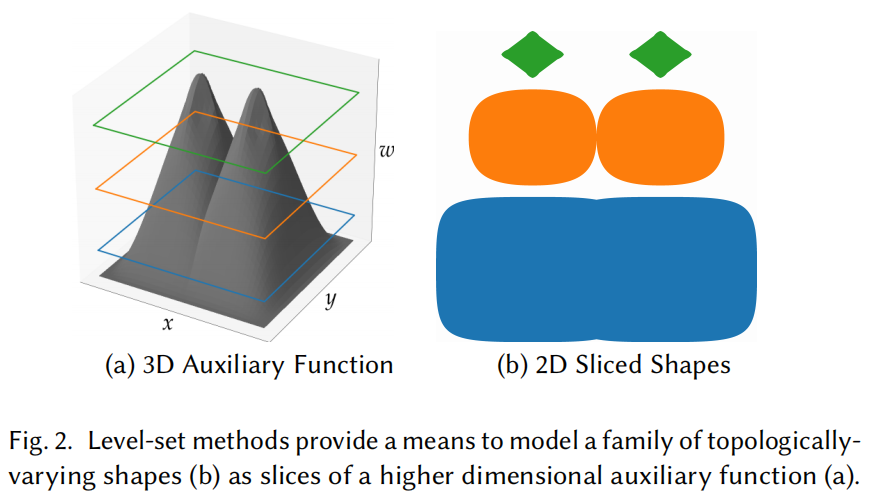
二. Level Set

为了表示拓扑变化中的复杂表面，Hypernerf 引入了 Level Set 方法，将复杂场景表面的拓扑变化表示为高维空间的切片：
$$\Gamma =\{(x,y,w)\mid S(x,y,w)=0\}$$

只需要使用不同的 $w_i$ 切片高维函数 $S$，就可以得到对应的二维形状 $\{(x,y)\mid S(x,y,w_i)=0\}$ 。

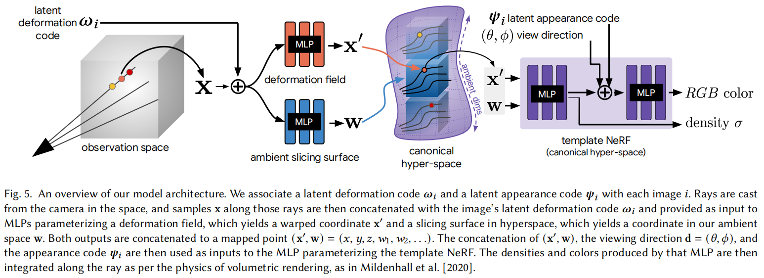
三. Hyper-Space Neural Radiance Fields

在 Nerfies 的基础上增加高维切片的 MLP，然后将其输出传入 Nerfies 的标准模板体：
$$\begin{array}{c}{\mathbf{x}}^{\prime }=T\left(\mathbf{x},{\omega }_i\right)\\ \mathbf{w}=H\left(\mathbf{x},{\omega }_i\right)\\ (\mathbf{c},\sigma )=F\left({\mathbf{x}}^{\prime },\mathbf{w},\mathbf{d},{\mathbf{\psi }}_i\right)\end{array}$$

D-Nerf

Neural Scene Flow Fields

Paper: Li Z, Niklaus S, Snavely N, et al. Neural scene flow fields for space-time view synthesis of dynamic scenes[C]//Proceedings of the IEEE/CVF Conference on Computer Vision and Pattern Recognition. 2021: 6498-6508.
Introduction: https://www.cs.cornell.edu/~zl548/NSFF/
Code: https://github.com/zhengqili/Neural-Scene-Flow-Fields

Neural Scene Flow Fields 是一种将 NeRF 扩展到动态场景的方法。它只需要输入一个单目 4D 视频，就可以重建出三维动态场景的外观、几何，以及三维场景中点的运动信息。

一. Neural scene flow fields

Neural Scene Flow Fields 的核心思想是利用场景流 (scene flow) 建模三维场景中每个点在每一时刻的运动向量场，通过训练一个神经场景流场 (Neural Scene Flow Fields) 来同时建模三维几何形状和其时间上的变化：
$$\left({\mathbf{c}}_i,{\sigma }_i,{\mathcal{F}}_i,{\mathcal{W}}_i\right)=F_{\Theta }^{\mathrm{dy}}(\mathbf{x},\mathbf{d},i)$$

其中 ${\mathcal{F}}_i=\left({\mathbf{f}}_{i\to i+1},{\mathbf{f}}_{i\to i-1}\right)$ 表示 $i$ 时刻 $\mathbf{x}$ 点的偏移向量，${\mathcal{W}}_i=\left(w_{i\to i+1},w_{i\to i-1}\right)$ 表示 $i$ 时刻 $\mathbf{x}$ 点的运动遮挡权重。

FPO

Paper: Wang L, Zhang J, Liu X, et al. Fourier plenoctrees for dynamic radiance field rendering in real-time[C]//Proceedings of the IEEE/CVF Conference on Computer Vision and Pattern Recognition. 2022: 13524-13534.
Introduction: https://aoliao12138.github.io/FPO/
Code: Unreleased

NeRFPlayer

Paper: Song L, Chen A, Li Z, et al. Nerfplayer: A streamable dynamic scene representation with decomposed neural radiance fields[J]. IEEE Transactions on Visualization and Computer Graphics, 2023, 29(5): 2732-2742.
Introduction: https://lsongx.github.io/projects/nerfplayer.html
Code: Unreleased

HexPlane

K-Planes

Paper: Fridovich-Keil S, Meanti G, Warburg F R, et al. K-planes: Explicit radiance fields in space, time, and appearance[C]//Proceedings of the IEEE/CVF Conference on Computer Vision and Pattern Recognition. 2023: 12479-12488.
Introduction: https://sarafridov.github.io/K-Planes/
Code: https://github.com/sarafridov/K-Planes

Tensor4D

Paper: Shao R, Zheng Z, Tu H, et al. Tensor4d: Efficient neural 4d decomposition for high-fidelity dynamic reconstruction and rendering[C]//Proceedings of the IEEE/CVF Conference on Computer Vision and Pattern Recognition. 2023: 16632-16642.
Introduction: https://liuyebin.com/tensor4d/tensor4d.html
Code: https://github.com/DSaurus/Tensor4D

HumanRF

Paper: Işık M, Rünz M, Georgopoulos M, et al. Humanrf: High-fidelity neural radiance fields for humans in motion[J]. ACM Transactions on Graphics (TOG), 2023, 42(4): 1-12.
Introduction: https://actors-hq.com/
Code: https://github.com/synthesiaresearch/humanrf

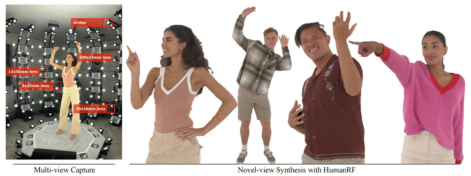
HumanRF 是一种基于 NeRF 的 4D 场景表示方法，能够根据输入的多视角同步视频重建出动态的全身人像，并保持高质量地渲染出任意视角的人物形态。为了高质量渲染逼真的人物形态，HumanRF 还采集了一个新的数据集 —— ActorsHQ。

一. 背景

根据现实世界中捕获的视频重建逼真的动态人像存在重大挑战：

1. 不同粒度的细节（如脸部、头发、衣着等）难以精准重建；
2. 快速和复杂的人体动作序列进一步加剧了重建的难度；

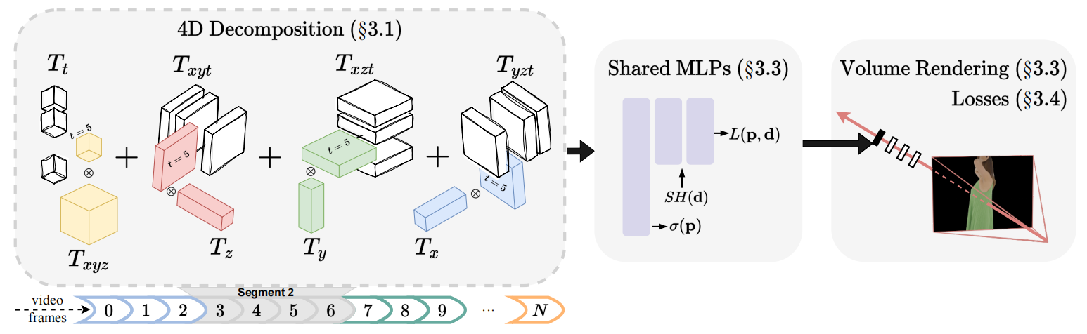
为了高质量地渲染出逼真的人物形态，HumanRF 采集了一个新的数据集 ActorsHQ，包含 8 个模特场景，每个场景 160 个机位，每个机位采集 3K × 4K 的高清视频。然后在新的数据集上，将三维 NeRF 场景表示扩展到时间维度，即将时间维与特征网格的时空低秩分解张量相结合。为了表示较长的时间序列，HumanRF 将输入视频分割成多段进行处理。

二. Adaptive Temporal Partitioning

使用一个单独的特征网络建模较长的时间序列效果远不如多个特征网络建模较短的时间序列，因此 HumanRF 将输入视频分割成多段分别处理。每段序列的分割长度在训练前使用一种贪心算法自适应获得。

三. 4D Feature Grid Decomposition

对于每一个分割后的 4D 视频序列 T ( k ) ∈ { t s , t s + 1 , t s + 2 , … , t s + N k − 1 } \mathcal{T}^{(k)} \in\left\{t_s, t_{s+1}, t_{s+2}, \ldots, t_{s+N_k-1}\right\} T(k)∈{ts​,ts+1​,ts+2​,…,ts+Nk​−1​}，训练一个 4D 特征网络 $T_{xyzt}^{(k)}:{\mathbb{R}}^4\mapsto {\mathbb{R}}^m$，能够将输入的查询点 ${\mathbf{p}}_{xyzt}$ 映射到 NeRF 的特征空间。在具体的 4D 表示中，将 4D 特征网络分解为 3D 特征网络和 1D 特征网络的乘积：
$$\begin{array}{rl}{T}_{xyzt}\left({\mathbf{p}}_{xyzt}\right)& =T_{xyz}\left({\mathbf{p}}_{xyz}\right)\odot T_t\left({\mathbf{p}}_t\right)\\ & +T_{xyt}\left({\mathbf{p}}_{xyt}\right)\odot T_z\left({\mathbf{p}}_z\right)\\ & +T_{xzt}\left({\mathbf{p}}_{xzt}\right)\odot T_y\left({\mathbf{p}}_y\right)\\ & +T_{yzt}\left({\mathbf{p}}_{yzt}\right)\odot T_x\left({\mathbf{p}}_x\right)\end{array}$$

其中 3D 特征网络 $\left(T_{xyz},T_{xyt},T_{xzt},T_{yzt}:{\mathbb{R}}^3\mapsto {\mathbb{R}}^m\right)$ 直接使用了 Instant-NGP，1D 特征网络 $\left(T_t,T_z,T_y,T_x:\mathbb{R}\mapsto {\mathbb{R}}^m\right)$ 就是简单的向量矩阵。

四. Shared MLPs and Volume Rendering

HumanRF 计算时刻 $t$ 在视角 $\mathbf{r}$ 处观察场景得到的颜色值的方法如下。体积密度和几何特征与空间位置和时间点有关：
{ σ ( p , t ) , F ( p , t ) } = MLP ⁡ σ ( T x y z t ( k ) ( p , t ) ) \{\sigma(\mathbf{p}, t), F(\mathbf{p}, t)\}=\operatorname{MLP}_\sigma\left(T_{x y z t}^{(k)}(\mathbf{p}, t)\right) {σ(p,t),F(p,t)}=MLPσ​(Txyzt(k)​(p,t))

颜色信息与视角、空间位置和时间点有关：
$$L(\mathbf{p},\mathbf{d},t)={\mathrm{MLP}}_L(\mathrm{SH}(\mathbf{d}),F(\mathbf{p},t))$$

然后仿照 NeRF 的 RGB 视图渲染策略进行分层抽样：
$$\hat{C}(\mathbf{r},t)={\int }_{{\alpha }_{\text{min }}}^{{\alpha }_{\max }}T(\alpha )\sigma (\mathbf{r}(\alpha ),t)L(\mathbf{r}(\alpha ),\mathrm{d},t)d\alpha$$

五. 训练

训练时使用原始 RGB 图像进行监督：
$$\begin{array}{rl}{\mathcal{L}}_{\text{pho }}& =\frac{1}{|\mathcal{R}|}\sum _{r\in \mathcal{R}}\{\begin{array}{ll}\frac{1}{2}{l}^2,& \text{ if }l\le \delta \\ \delta \cdot \left(l-\frac{1}{2}\delta \right),& \text{ otherwise }\end{array}\\ & \text{where }l=\left|C(\mathbf{r},t)-\hat{C}(\mathbf{r},t)\right|\end{array}$$

为了加速早期的训练过程，还引入了 mask 损失以优化不透明度：
$$\begin{array}{rl}{\mathcal{L}}_{\text{bce }}& =\frac{1}{|\mathcal{R}|}\sum _{\mathbf{r}\in \mathcal{R}}[M(\mathbf{r})\log (\hat{M}(\mathbf{r}))+(1-M(\mathbf{r}))\log ((\hat{M}(\mathbf{r}))]\\ & \text{where }\hat{M}(\mathbf{r})={\int }_{{\alpha }_{\min }}^{{\alpha }_{\max }}T(\alpha )\sigma (\mathbf{r}(\alpha ))d\alpha \end{array}$$

因此总的损失函数如下：
$$\mathcal{L}={\mathcal{L}}_{\text{pho }}+\beta {\mathcal{L}}_{\text{bce }}$$