扩散模型的系统性学习（一）：DDPM的学习

一、学习的资料

我们需要直接找相关的论文，以及其代码的相关实现，才能更好的去理解这个模型的原理以及实现是怎样的。
之前的学习过程之寻找了代码，然后寻找了很多零零散散的二次加工资料来进行学习，导致整个学习的过程比较杂乱，效率低下。
我们需要寻找的参考资料，比如论文和实现代码这些，必须是一手的，而不是加工过的二次生产的；
而对于帮助理解原理的资料，为了我们能更的理解，我们可以选择加工过的更适合我们理解相关概念的资料。

以下是我在这个过程当中用到的资料，包括论文公式的解读，代码的实现等：

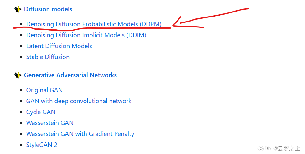
1.1 对于扩散模型的发展过程的综述

参考这里的发展流程去系统性的学习扩散模型
扩散模型汇总——从DDPM到DALLE2

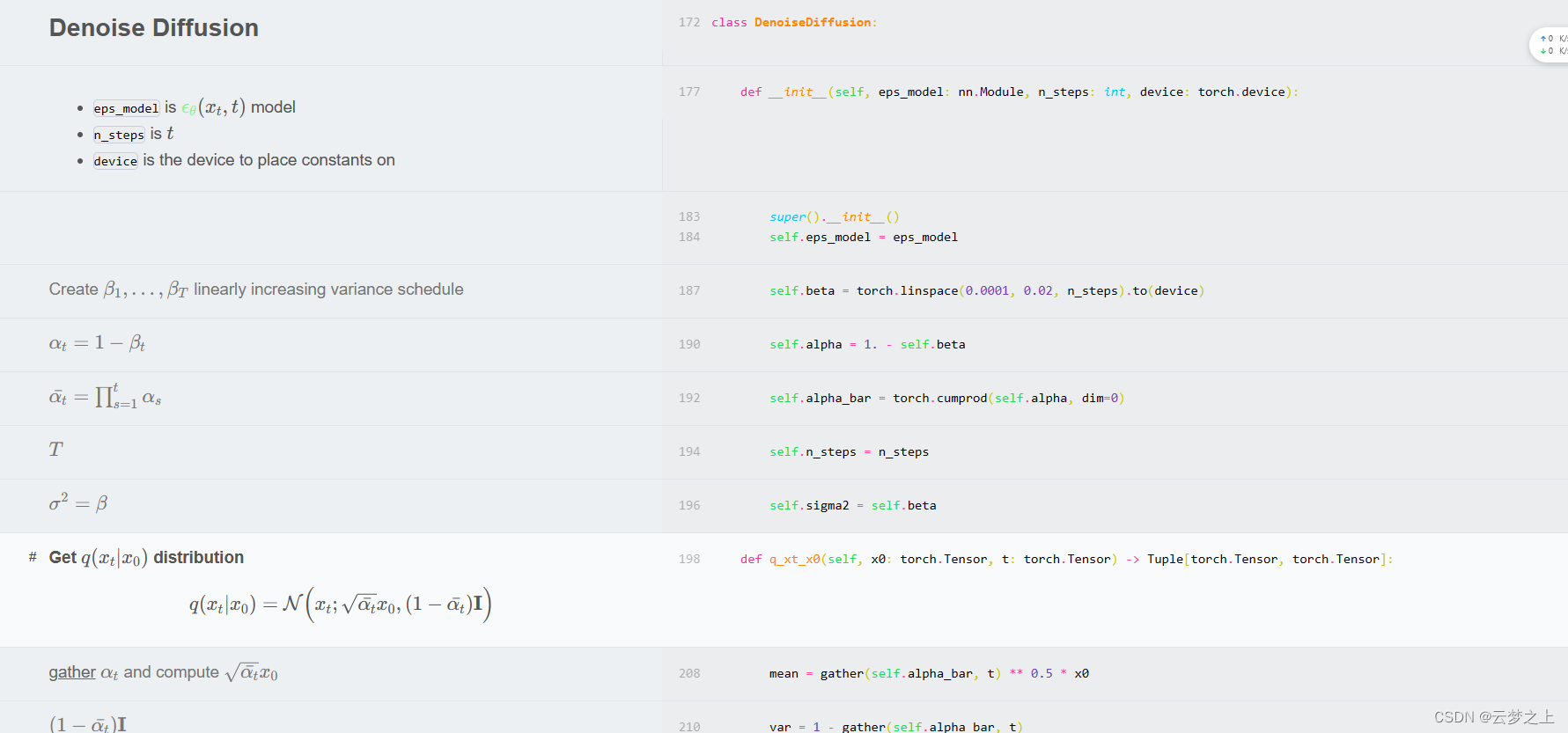
1.2对论文中涉及的公式以及公式对应的代码的解读

对论文中涉及的公式以及公式对应的代码的解读

可以看到这里面有对于论文当中涉及公式内容的实现，帮助我们理解代码和公式之间的关系

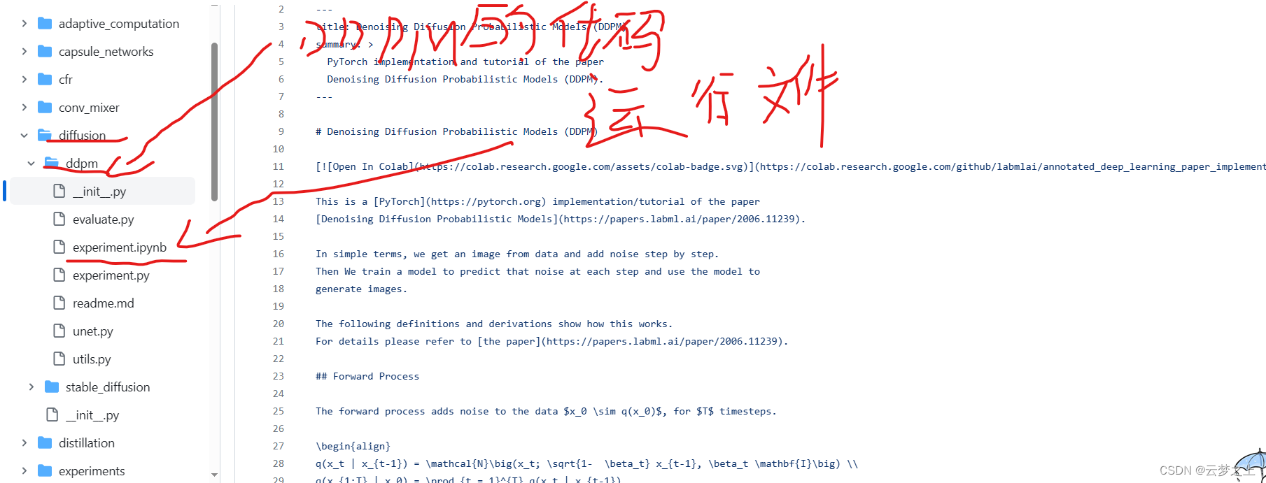
1.3github中对于各模型实现的代码

github中对于各模型实现的代码
可以看到这个网站包含了很多网络的实现代码，以及程序运行的代码文件，我们可以结合①②网页一起去学习一个模型

1.4相关基础知识的学习

transformer的粗略学习

二、DDPM的学习

2.1 DDPM总体知识的梳理

整个DDPM网络架构的设计
    高斯扩散模型的结构
        前向加噪过程
            输入x0，和t，计算出xt

        反向采样的过程
            给定xt，和t，求第t步的值（t为我们希望取样得到的加入噪声t步后的图像））
            我们首先通过unet网路，求得我们在x0时刻加入的噪声ε
            然后有噪声ε和xt，我们可以反向求得x0（即为原图）
            然后我们在随机生成一个正太分布N，然后利用x0和N进行正向的采样加噪得到xt

        损失函数的计算
            对于每批次的图片（x0）我们随机生成一个时间t，和一个正太分布N
            我们用前向传播计算第t加噪后的图像xt
            然后我们用unet网络，输入xt和t，然后去预测我们在x0生成xt时所使用的正太分布N，预测结果为ε
            最后去计算实际用的N与预测的ε之间的损失，用来进行梯度的更新
            这样设计损失函数的作用
                让我们的unet模型能够根据给定的xt，去生成x0时刻加的噪声ε为多少，然后我们就可以通过公式由（ε，和xt）去反向的计算x0（也就是计算出原图）

    unet的网络的结构
        整个模块的示意图
        各模块的设计
            时间嵌入模块
                将时间t的维度转化为n维，一般维度为sin，另一半维度为cos

            残差模块
                将输入的x和时间嵌入t进行融合，从而让我们的图像它具有了时间步骤信息
                同时也进行了channel的变化

            注意力模块
                只对x进行操作，通过注意力机制，在原本的x中，加入了一张图中各小图片块之间的相关性信息

            下采样模块
                采用res块（对x增加t的信息）
                采用atte块（在某些块里增加）

            下采样
                进行卷积操作，不改变维度，减少图片的长宽

            上采样模块
                采用res块（对x增加t的信息）
                采用atte块（在某些块里增加）

            上采样
                进行反向卷积操作，不改变维度，增加图片的长宽


        预测过程的实现
            我们在下采样阶段会记录每次采样后的结果，用于后续上采样阶段时还原我们的原始图像（也就是我们的上采样的结果不是随机生成的，而是在原来的基础上，加上我们的模型学到的一些东西，让我们的unet网络可以实现对原始图像的一定程度的还原）

        作用
            unet做的事情是预测我们在正向加噪阶段加入的正太分布噪声ε



整个训练流程的设计
    train
        对于每个批次
            随机生成时间步骤t
            利用原图（x0）和t，以及随机生成的正太分布N，进行前向采样得到xt
            利用unet，对采样得到xt，和t，进行预测得到在x0时加噪用的噪声的预测值ε
            然后计算ε和实际加噪的N的损失值进行梯度更新


    sample
        当我们训练好了Unet网络之后，我们就可以利用unet网络进行反向迭代去噪
        t从第999步开始到0
            首先输入一个随机生成的正太分布N,当做x999.
            然后利用unet网络（x999,999），生成x0加入的噪声ε
            然后利用x999和ε，计算出x0,
            然后用x0，和再一次随机生成的N，进行前向传播，计算出x999作为下一次的输入的x

        最后我们一步步迭代，指导从x0到0，既得到原图

2.2相关代码的解读

2.2.1unet 代码块

"""
---
title: U-Net model for Denoising Diffusion Probabilistic Models (DDPM)
summary: >
  UNet model for Denoising Diffusion Probabilistic Models (DDPM)
---

# U-Net model for [Denoising Diffusion Probabilistic Models (DDPM)](index.html)

This is a [U-Net](../../unet/index.html) based model to predict noise
$\textcolor{lightgreen}{\epsilon_\theta}(x_t, t)$.

U-Net is a gets it's name from the U shape in the model diagram.
It processes a given image by progressively lowering (halving) the feature map resolution and then
increasing the resolution.
There are pass-through connection at each resolution.

![U-Net diagram from paper](../../unet/unet.png)

This implementation contains a bunch of modifications to original U-Net (residual blocks, multi-head attention)
 and also adds time-step embeddings $t$.
"""

import math
from typing import Optional, Tuple, Union, List

import torch
from torch import nn

from labml_helpers.module import Module


class Swish(Module):
    """
    ### Swish actiavation function

    $$x \cdot \sigma(x)$$
    """

    def forward(self, x):
        return x * torch.sigmoid(x)


class TimeEmbedding(nn.Module):
    """
    ### Embeddings for $t$
    """

    def __init__(self, n_channels: int):
        """
        * `n_channels` is the number of dimensions in the embedding
        """
        super().__init__()
        self.n_channels = n_channels
        # First linear layer
        self.lin1 = nn.Linear(self.n_channels // 4, self.n_channels)
        # Activation
        self.act = Swish()
        # Second linear layer
        self.lin2 = nn.Linear(self.n_channels, self.n_channels)

    def forward(self, t: torch.Tensor):
        # Create sinusoidal position embeddings
        # [same as those from the transformer](../../transformers/positional_encoding.html)
        #
        # \begin{align}
        # PE^{(1)}_{t,i} &= sin\Bigg(\frac{t}{10000^{\frac{i}{d - 1}}}\Bigg) \\
        # PE^{(2)}_{t,i} &= cos\Bigg(\frac{t}{10000^{\frac{i}{d - 1}}}\Bigg)
        # \end{align}
        #
        # where $d$ is `half_dim`
        #初始化的n_channels为64*4，这里half_dim为32
        half_dim = self.n_channels // 8
        emb = math.log(10_000) / (half_dim - 1)
        emb = torch.exp(torch.arange(half_dim, device=t.device) * -emb)
        #这里t的行不变，增加列维度为1；额，emb的列不变，行变为1
        #两者相乘得到（t，emb）的举证
        emb = t[:, None] * emb[None, :]
        emb = torch.cat((emb.sin(), emb.cos()), dim=1)
        #最后emb变为了64
        # Transform with the MLP
        #通过lin1维度转化为了64*4  也就是n_channels*4
        emb = self.act(self.lin1(emb))
        emb = self.lin2(emb)

        #
        return emb

#残差块的作用是将原始数据和进行了位置信息嵌入的时间步骤t进行融合
class ResidualBlock(Module):
    """
    ### Residual block

    A residual block has two convolution layers with group normalization.
    Each resolution is processed with two residual blocks.
    """
    #残差块的初始化要指定输入、输出、和时间嵌入的通道数3个变量
    def __init__(self, in_channels: int, out_channels: int, time_channels: int,
                 n_groups: int = 32, dropout: float = 0.1):
        """
        * `in_channels` is the number of input channels
        * `out_channels` is the number of input channels
        * `time_channels` is the number channels in the time step ($t$) embeddings
        * `n_groups` is the number of groups for [group normalization](../../normalization/group_norm/index.html)
        * `dropout` is the dropout rate
        """
        super().__init__()
        # Group normalization and the first convolution layer
        self.norm1 = nn.GroupNorm(n_groups, in_channels)
        self.act1 = Swish()
        self.conv1 = nn.Conv2d(in_channels, out_channels, kernel_size=(3, 3), padding=(1, 1))

        # Group normalization and the second convolution layer
        self.norm2 = nn.GroupNorm(n_groups, out_channels)
        self.act2 = Swish()
        self.conv2 = nn.Conv2d(out_channels, out_channels, kernel_size=(3, 3), padding=(1, 1))

        # If the number of input channels is not equal to the number of output channels we have to
        # project the shortcut connection
        if in_channels != out_channels:
            self.shortcut = nn.Conv2d(in_channels, out_channels, kernel_size=(1, 1))
        else:
            self.shortcut = nn.Identity()

        # Linear layer for time embeddings
        self.time_emb = nn.Linear(time_channels, out_channels)
        self.time_act = Swish()

        self.dropout = nn.Dropout(dropout)

    def forward(self, x: torch.Tensor, t: torch.Tensor):
        """
        * `x` has shape `[batch_size, in_channels, height, width]`
        * `t` has shape `[batch_size, time_channels]`
        """
        # First convolution layer
        h = self.conv1(self.act1(self.norm1(x)))
        # Add time embeddings
        #将t先进性激活，然后进行位置嵌入，然后进行维度扩充，然后和h相加
        h += self.time_emb(self.time_act(t))[:, :, None, None]
        # Second convolution layer
        h = self.conv2(self.dropout(self.act2(self.norm2(h))))

        # Add the shortcut connection and return
        return h + self.shortcut(x)




##注意力模块单独的只对x进行操作，增强x的中上下文的关联信息（输入的x为已经加入了位置嵌入信息的x）
class AttentionBlock(Module):
    """
    ### Attention block

    This is similar to [transformer multi-head attention](../../transformers/mha.html).
    """
    #注意力块的初始化只要指定一个n_channels的大小
    # 定义类的初始化方法
    def __init__(self, n_channels: int, n_heads: int = 1, d_k: int = None, n_groups: int = 32):
        """
        * `n_channels` is the number of channels in the input
        * `n_heads` is the number of heads in multi-head attention
        * `d_k` is the number of dimensions in each head
        * `n_groups` is the number of groups for group normalization
        """
        # 调用父类的初始化方法
        super().__init__()

        # 如果没有指定`d_k`，则将其设置为与输入通道数相同
        if d_k is None:
            d_k = n_channels
        # 创建一个组归一化层，用于对输入进行归一化处理
        self.norm = nn.GroupNorm(n_groups, n_channels)
        # 创建一个线性层，用于生成查询、键和值
        self.projection = nn.Linear(n_channels, n_heads * d_k * 3)
        # 创建一个线性层，用于最后的变换
        self.output = nn.Linear(n_heads * d_k, n_channels)
        # 计算点积注意力的缩放因子
        self.scale = d_k ** -0.5
        #
        self.n_heads = n_heads
        self.d_k = d_k

    def forward(self, x: torch.Tensor, t: Optional[torch.Tensor] = None):
        """
        * `x` has shape `[batch_size, in_channels, height, width]`
        * `t` has shape `[batch_size, time_channels]`
        """
        # `t` is not used, but it's kept in the arguments because for the attention layer function signature
        # to match with `ResidualBlock`.
        _ = t
        # Get shape
        batch_size, n_channels, height, width = x.shape
        # Change `x` to shape `[batch_size, seq, n_channels]`
        x = x.view(batch_size, n_channels, -1).permute(0, 2, 1)
        # Get query, key, and values (concatenated) and shape it to `[batch_size, seq, n_heads, 3 * d_k]`
        #只是通道数在改变，中间的-1表示，每个矩阵的像素
        qkv = self.projection(x).view(batch_size, -1, self.n_heads, 3 * self.d_k)
        #这里DK相当于是把，每张图片的一个维度划分为dk块，然后，每个块里面的数据的大小就为-1数值的值
        # Split query, key, and values. Each of them will have shape `[batch_size, seq, n_heads, d_k]`、
        #q, k, v = torch.chunk(qkv, 3, dim=-1)
        #这行代码的作用是将输入张量qkv沿着最后一个维度均匀地分割成3个张量块，并分别赋值给q、k和v。
        q, k, v = torch.chunk(qkv, 3, dim=-1)
        # Calculate scaled dot-product $\frac{Q K^\top}{\sqrt{d_k}}$
        attn = torch.einsum('bihd,bjhd->bijh', q, k) * self.scale
        # Softmax along the sequence dimension $\underset{seq}{softmax}\Bigg(\frac{Q K^\top}{\sqrt{d_k}}\Bigg)$
        attn = attn.softmax(dim=2)
        # Multiply by values
        res = torch.einsum('bijh,bjhd->bihd', attn, v)
        # Reshape to `[batch_size, seq, n_heads * d_k]`
        res = res.view(batch_size, -1, self.n_heads * self.d_k)
        # Transform to `[batch_size, seq, n_channels]`
        res = self.output(res)

        # Add skip connection
        res += x

        # Change to shape `[batch_size, in_channels, height, width]`
        res = res.permute(0, 2, 1).view(batch_size, n_channels, height, width)

        #
        return res


class DownBlock(Module):
    """
    ### Down block

    This combines `ResidualBlock` and `AttentionBlock`. These are used in the first half of U-Net at each resolution.
    """

    def __init__(self, in_channels: int, out_channels: int, time_channels: int, has_attn: bool):
        super().__init__()
        self.res = ResidualBlock(in_channels, out_channels, time_channels)
        if has_attn:
            self.attn = AttentionBlock(out_channels)
        else:
            #nn.Identity()是一个特殊的模块，它不对输入数据进行任何操作或变换，而是直接返回输入的数
            self.attn = nn.Identity()

    def forward(self, x: torch.Tensor, t: torch.Tensor):
        x = self.res(x, t)
        x = self.attn(x)
        return x

#上块，和之前的下块相反，在开始2块加入注意力，然后在最后一层不进行上采样
class UpBlock(Module):
    """
    ### Up block

    This combines `ResidualBlock` and `AttentionBlock`. These are used in the second half of U-Net at each resolution.
    """

    def __init__(self, in_channels: int, out_channels: int, time_channels: int, has_attn: bool):
        super().__init__()
        # The input has `in_channels + out_channels` because we concatenate the output of the same resolution
        # from the first half of the U-Net
        self.res = ResidualBlock(in_channels + out_channels, out_channels, time_channels)
        if has_attn:
            self.attn = AttentionBlock(out_channels)
        else:
            self.attn = nn.Identity()

    def forward(self, x: torch.Tensor, t: torch.Tensor):
        x = self.res(x, t)
        x = self.attn(x)
        return x


#中间层为残差连接+注意力块+残差连接
class MiddleBlock(Module):
    """
    ### Middle block

    It combines a `ResidualBlock`, `AttentionBlock`, followed by another `ResidualBlock`.
    This block is applied at the lowest resolution of the U-Net.
    """

    def __init__(self, n_channels: int, time_channels: int):
        super().__init__()
        self.res1 = ResidualBlock(n_channels, n_channels, time_channels)
        self.attn = AttentionBlock(n_channels)
        self.res2 = ResidualBlock(n_channels, n_channels, time_channels)

    def forward(self, x: torch.Tensor, t: torch.Tensor):
        x = self.res1(x, t)
        x = self.attn(x)
        x = self.res2(x, t)
        return x


#上采样块，实现反向局卷积，对原始的维度进行还原
class Upsample(nn.Module):
    """
    ### Scale up the feature map by $2 \times$
    """
    #创建了一个二维转置卷积层，用于上采样
    def __init__(self, n_channels):
        super().__init__()
        self.conv = nn.ConvTranspose2d(n_channels, n_channels, (4, 4), (2, 2), (1, 1))

    def forward(self, x: torch.Tensor, t: torch.Tensor):
        # `t` is not used, but it's kept in the arguments because for the attention layer function signature
        # to match with `ResidualBlock`.
        _ = t
        return self.conv(x)


#下采样实际上做的就是局昂及操作，让每层的分辨率的大小降低，而维度并不发生变化
class Downsample(nn.Module):
    """
    ### Scale down the feature map by $\frac{1}{2} \times$
    """

    def __init__(self, n_channels):
        super().__init__()
        #参数可以是一个整数或者一个二元组。
        #如果是一个整数，那么卷积核的高度和宽度都是这个值；
        #如果是一个二元组，那么卷积核的高度和宽度可以分别设置。
        #(3, 3): 表示卷积核的大小在高度和宽度上都是3。
        #（2，2): 表示卷积的步长在高度和宽度上都是2。
        #（1，1): 表示输入数据的填充大小在高度和宽度上都是1
        self.conv = nn.Conv2d(n_channels, n_channels, (3, 3), (2, 2), (1, 1))

    def forward(self, x: torch.Tensor, t: torch.Tensor):
        # `t` is not used, but it's kept in the arguments because for the attention layer function signature
        # to match with `ResidualBlock`.
        _ = t
        return self.conv(x)


class UNet(Module):
    """
    ## U-Net
    """
    #Union[Tuple[int, ...], List[int]]表示ch_mults参数可以是一个元组或列表，其中元素的类型为整数。
    def __init__(self, image_channels: int = 3, n_channels: int = 64,
                 ch_mults: Union[Tuple[int, ...], List[int]] = (1, 2, 2, 4),
                 is_attn: Union[Tuple[bool, ...], List[int]] = (False, False, True, True),
                 n_blocks: int = 2):
        """
        * `image_channels` is the number of channels in the image. $3$ for RGB.
        * `n_channels` is number of channels in the initial feature map that we transform the image into
        * `ch_mults` is the list of channel numbers at each resolution. The number of channels is `ch_mults[i] * n_channels`
        * `is_attn` is a list of booleans that indicate whether to use attention at each resolution
        * `n_blocks` is the number of `UpDownBlocks` at each resolution
        """
        super().__init__()

        # Number of resolutions
        n_resolutions = len(ch_mults)

        # Project image into feature map
        self.image_proj = nn.Conv2d(image_channels, n_channels, kernel_size=(3, 3), padding=(1, 1))

        # Time embedding layer. Time embedding has `n_channels * 4` channels
        self.time_emb = TimeEmbedding(n_channels * 4)

        # #### First half of U-Net - decreasing resolution
        down = []
        # Number of channels
        out_channels = in_channels = n_channels
        # For each resolution
        #对于4层
        for i in range(n_resolutions):
            # Number of output channels at this resolution
            out_channels = in_channels * ch_mults[i]
            # Add `n_blocks`
            #每层2快，一块进行残差引入位置t的嵌入信息，以及在某些时候引入注意力信息 ，另一块进行下采样
            for _ in range(n_blocks):
                down.append(DownBlock(in_channels, out_channels, n_channels * 4, is_attn[i]))
                in_channels = out_channels
            # Down sample at all resolutions except the last
            if i < n_resolutions - 1:
                down.append(Downsample(in_channels))
        #将一个模块列表（可能是一系列的卷积层、池化层等）封装成一个nn.ModuleList。
        #nn.ModuleList是PyTorch中的一个类，它可以包含一系列的模块，并且可以像Python的列表一样进行索引。
        # 当你把一系列模块放入nn.ModuleList后，这些模块就会被正确地注册为网络的一部分，
        # 从而能够正确地进行前向传播和反向传播
        # Combine the set of modules
        self.down = nn.ModuleList(down)

        # Middle block
        self.middle = MiddleBlock(out_channels, n_channels * 4, )

        # #### Second half of U-Net - increasing resolution
        up = []
        # Number of channels
        in_channels = out_channels
        # For each resolution
        for i in reversed(range(n_resolutions)):
            # `n_blocks` at the same resolution
            out_channels = in_channels
            for _ in range(n_blocks):
                up.append(UpBlock(in_channels, out_channels, n_channels * 4, is_attn[i]))
            # Final block to reduce the number of channels
            out_channels = in_channels // ch_mults[i]
            up.append(UpBlock(in_channels, out_channels, n_channels * 4, is_attn[i]))
            in_channels = out_channels
            # Up sample at all resolutions except last
            if i > 0:
                up.append(Upsample(in_channels))

        # Combine the set of modules
        self.up = nn.ModuleList(up)

        # Final normalization and convolution layer
        self.norm = nn.GroupNorm(8, n_channels)
        self.act = Swish()
        self.final = nn.Conv2d(in_channels, image_channels, kernel_size=(3, 3), padding=(1, 1))

    def forward(self, x: torch.Tensor, t: torch.Tensor):
        """
        * `x` has shape `[batch_size, in_channels, height, width]`
        * `t` has shape `[batch_size]`
        """

        # Get time-step embeddings
        t = self.time_emb(t)

        # Get image projection
        x = self.image_proj(x)

        # `h` will store outputs at each resolution for skip connection
        h = [x]
        # First half of U-Net
        for m in self.down:
            x = m(x, t)
            h.append(x)

        # Middle (bottom)
        x = self.middle(x, t)

        # Second half of U-Net
        for m in self.up:
            #如果是上采样，那么我们进行上采样计算，同时更新我们的x
            if isinstance(m, Upsample):
                x = m(x, t)
            else:
                # Get the skip connection from first half of U-Net and concatenate
                #如果不是上采样，那么我们进行上采样块的计算，这里就需要用到下采样时记录的x，
                # 用来让我们上采样生成的图片更加的接近我们的原始图像，而不是随机生成的
                s = h.pop()
                #(batch_size, n_channels, height, width)
                #第2个通道数是n_channels  ，所以这里是把维数进行了一个扩充
                x = torch.cat((x, s), dim=1)

                x = m(x, t)

        # Final normalization and convolution
        #最后的final让维度重新回归为image_channels的3
        return self.final(self.act(self.norm(x)))

2.2.2高斯扩散代码块

"""
---
title: Denoising Diffusion Probabilistic Models (DDPM)
summary: >
  PyTorch implementation and tutorial of the paper
  Denoising Diffusion Probabilistic Models (DDPM).
---

# Denoising Diffusion Probabilistic Models (DDPM)

[![Open In Colab](https://colab.research.google.com/assets/colab-badge.svg)](https://colab.research.google.com/github/labmlai/annotated_deep_learning_paper_implementations/blob/master/labml_nn/diffusion/ddpm/experiment.ipynb)

This is a [PyTorch](https://pytorch.org) implementation/tutorial of the paper
[Denoising Diffusion Probabilistic Models](https://papers.labml.ai/paper/2006.11239).

In simple terms, we get an image from data and add noise step by step.
Then We train a model to predict that noise at each step and use the model to
generate images.

The following definitions and derivations show how this works.
For details please refer to [the paper](https://papers.labml.ai/paper/2006.11239).

## Forward Process

The forward process adds noise to the data $x_0 \sim q(x_0)$, for $T$ timesteps.

\begin{align}
q(x_t | x_{t-1}) = \mathcal{N}\big(x_t; \sqrt{1-  \beta_t} x_{t-1}, \beta_t \mathbf{I}\big) \\
q(x_{1:T} | x_0) = \prod_{t = 1}^{T} q(x_t | x_{t-1})
\end{align}

where $\beta_1, \dots, \beta_T$ is the variance schedule.

We can sample $x_t$ at any timestep $t$ with,

\begin{align}
q(x_t|x_0) &= \mathcal{N} \Big(x_t; \sqrt{\bar\alpha_t} x_0, (1-\bar\alpha_t) \mathbf{I} \Big)
\end{align}

where $\alpha_t = 1 - \beta_t$ and $\bar\alpha_t = \prod_{s=1}^t \alpha_s$

## Reverse Process

The reverse process removes noise starting at $p(x_T) = \mathcal{N}(x_T; \mathbf{0}, \mathbf{I})$
for $T$ time steps.

\begin{align}
\textcolor{lightgreen}{p_\theta}(x_{t-1} | x_t) &= \mathcal{N}\big(x_{t-1};
 \textcolor{lightgreen}{\mu_\theta}(x_t, t), \textcolor{lightgreen}{\Sigma_\theta}(x_t, t)\big) \\
\textcolor{lightgreen}{p_\theta}(x_{0:T}) &= \textcolor{lightgreen}{p_\theta}(x_T) \prod_{t = 1}^{T} \textcolor{lightgreen}{p_\theta}(x_{t-1} | x_t) \\
\textcolor{lightgreen}{p_\theta}(x_0) &= \int \textcolor{lightgreen}{p_\theta}(x_{0:T}) dx_{1:T}
\end{align}

$\textcolor{lightgreen}\theta$ are the parameters we train.

## Loss

We optimize the ELBO (from Jenson's inequality) on the negative log likelihood.

\begin{align}
\mathbb{E}[-\log \textcolor{lightgreen}{p_\theta}(x_0)]
 &\le \mathbb{E}_q [ -\log \frac{\textcolor{lightgreen}{p_\theta}(x_{0:T})}{q(x_{1:T}|x_0)} ] \\
 &=L
\end{align}

The loss can be rewritten as  follows.

\begin{align}
L
 &= \mathbb{E}_q [ -\log \frac{\textcolor{lightgreen}{p_\theta}(x_{0:T})}{q(x_{1:T}|x_0)} ] \\
 &= \mathbb{E}_q [ -\log p(x_T) - \sum_{t=1}^T \log \frac{\textcolor{lightgreen}{p_\theta}(x_{t-1}|x_t)}{q(x_t|x_{t-1})} ] \\
 &= \mathbb{E}_q [
  -\log \frac{p(x_T)}{q(x_T|x_0)}
  -\sum_{t=2}^T \log \frac{\textcolor{lightgreen}{p_\theta}(x_{t-1}|x_t)}{q(x_{t-1}|x_t,x_0)}
  -\log \textcolor{lightgreen}{p_\theta}(x_0|x_1)] \\
 &= \mathbb{E}_q [
   D_{KL}(q(x_T|x_0) \Vert p(x_T))
  +\sum_{t=2}^T D_{KL}(q(x_{t-1}|x_t,x_0) \Vert \textcolor{lightgreen}{p_\theta}(x_{t-1}|x_t))
  -\log \textcolor{lightgreen}{p_\theta}(x_0|x_1)]
\end{align}

$D_{KL}(q(x_T|x_0) \Vert p(x_T))$ is constant since we keep $\beta_1, \dots, \beta_T$ constant.

### Computing $L_{t-1} = D_{KL}(q(x_{t-1}|x_t,x_0) \Vert \textcolor{lightgreen}{p_\theta}(x_{t-1}|x_t))$

The forward process posterior conditioned by $x_0$ is,

\begin{align}
q(x_{t-1}|x_t, x_0) &= \mathcal{N} \Big(x_{t-1}; \tilde\mu_t(x_t, x_0), \tilde\beta_t \mathbf{I} \Big) \\
\tilde\mu_t(x_t, x_0) &= \frac{\sqrt{\bar\alpha_{t-1}}\beta_t}{1 - \bar\alpha_t}x_0
                         + \frac{\sqrt{\alpha_t}(1 - \bar\alpha_{t-1})}{1-\bar\alpha_t}x_t \\
\tilde\beta_t &= \frac{1 - \bar\alpha_{t-1}}{1 - \bar\alpha_t} \beta_t
\end{align}

The paper sets $\textcolor{lightgreen}{\Sigma_\theta}(x_t, t) = \sigma_t^2 \mathbf{I}$ where $\sigma_t^2$ is set to constants
$\beta_t$ or $\tilde\beta_t$.

Then,
$$\textcolor{lightgreen}{p_\theta}(x_{t-1} | x_t) = \mathcal{N}\big(x_{t-1}; \textcolor{lightgreen}{\mu_\theta}(x_t, t), \sigma_t^2 \mathbf{I} \big)$$

For given noise $\epsilon \sim \mathcal{N}(\mathbf{0}, \mathbf{I})$ using $q(x_t|x_0)$

\begin{align}
x_t(x_0, \epsilon) &= \sqrt{\bar\alpha_t} x_0 + \sqrt{1-\bar\alpha_t}\epsilon \\
x_0 &= \frac{1}{\sqrt{\bar\alpha_t}} \Big(x_t(x_0, \epsilon) -  \sqrt{1-\bar\alpha_t}\epsilon\Big)
\end{align}

This gives,

\begin{align}
L_{t-1}
 &= D_{KL}(q(x_{t-1}|x_t,x_0) \Vert \textcolor{lightgreen}{p_\theta}(x_{t-1}|x_t)) \\
 &= \mathbb{E}_q \Bigg[ \frac{1}{2\sigma_t^2}
 \Big \Vert \tilde\mu(x_t, x_0) - \textcolor{lightgreen}{\mu_\theta}(x_t, t) \Big \Vert^2 \Bigg] \\
 &= \mathbb{E}_{x_0, \epsilon} \Bigg[ \frac{1}{2\sigma_t^2}
  \bigg\Vert \frac{1}{\sqrt{\alpha_t}} \Big(
  x_t(x_0, \epsilon) - \frac{\beta_t}{\sqrt{1 - \bar\alpha_t}} \epsilon
  \Big) - \textcolor{lightgreen}{\mu_\theta}(x_t(x_0, \epsilon), t) \bigg\Vert^2 \Bigg] \\
\end{align}

Re-parameterizing with a model to predict noise

\begin{align}
\textcolor{lightgreen}{\mu_\theta}(x_t, t) &= \tilde\mu \bigg(x_t,
  \frac{1}{\sqrt{\bar\alpha_t}} \Big(x_t -
   \sqrt{1-\bar\alpha_t}\textcolor{lightgreen}{\epsilon_\theta}(x_t, t) \Big) \bigg) \\
  &= \frac{1}{\sqrt{\alpha_t}} \Big(x_t -
  \frac{\beta_t}{\sqrt{1-\bar\alpha_t}}\textcolor{lightgreen}{\epsilon_\theta}(x_t, t) \Big)
\end{align}

where $\epsilon_\theta$ is a learned function that predicts $\epsilon$ given $(x_t, t)$.

This gives,

\begin{align}
L_{t-1}
&= \mathbb{E}_{x_0, \epsilon} \Bigg[ \frac{\beta_t^2}{2\sigma_t^2 \alpha_t (1 - \bar\alpha_t)}
  \Big\Vert
  \epsilon - \textcolor{lightgreen}{\epsilon_\theta}(\sqrt{\bar\alpha_t} x_0 + \sqrt{1-\bar\alpha_t}\epsilon, t)
  \Big\Vert^2 \Bigg]
\end{align}

That is, we are training to predict the noise.

### Simplified loss

$$L_{\text{simple}}(\theta) = \mathbb{E}_{t,x_0, \epsilon} \Bigg[ \bigg\Vert
\epsilon - \textcolor{lightgreen}{\epsilon_\theta}(\sqrt{\bar\alpha_t} x_0 + \sqrt{1-\bar\alpha_t}\epsilon, t)
\bigg\Vert^2 \Bigg]$$

This minimizes $-\log \textcolor{lightgreen}{p_\theta}(x_0|x_1)$ when $t=1$ and $L_{t-1}$ for $t\gt1$ discarding the
weighting in $L_{t-1}$. Discarding the weights $\frac{\beta_t^2}{2\sigma_t^2 \alpha_t (1 - \bar\alpha_t)}$
increase the weight given to higher $t$ (which have higher noise levels), therefore increasing the sample quality.

This file implements the loss calculation and a basic sampling method that we use to generate images during
training.

Here is the [UNet model](unet.html) that gives $\textcolor{lightgreen}{\epsilon_\theta}(x_t, t)$ and
[training code](experiment.html).
[This file](evaluate.html) can generate samples and interpolations from a trained model.
"""
from typing import Tuple, Optional

import torch
import torch.nn.functional as F
import torch.utils.data
from torch import nn

from labml_nn.diffusion.ddpm.utils import gather



###详细的对于扩散模型的代码和公式的对应请看以下网页中的内容：https://nn.labml.ai/diffusion/ddpm/index.html
class DenoiseDiffusion:
    """
    ## Denoise Diffusion
    """

    def __init__(self, eps_model: nn.Module, n_steps: int, device: torch.device):
        """
        * `eps_model` is $\textcolor{lightgreen}{\epsilon_\theta}(x_t, t)$ model
        * `n_steps` is $t$
        * `device` is the device to place constants on
        """
        super().__init__()
        self.eps_model = eps_model

        # Create $\beta_1, \dots, \beta_T$ linearly increasing variance schedule
        self.beta = torch.linspace(0.0001, 0.02, n_steps).to(device)

        # $\alpha_t = 1 - \beta_t$
        self.alpha = 1. - self.beta
        # $\bar\alpha_t = \prod_{s=1}^t \alpha_s$
        self.alpha_bar = torch.cumprod(self.alpha, dim=0)
        # $T$
        self.n_steps = n_steps
        # $\sigma^2 = \beta$
        self.sigma2 = self.beta

        ##->箭头右边的 表示函数返回类型的注释
    def q_xt_x0(self, x0: torch.Tensor, t: torch.Tensor) -> Tuple[torch.Tensor, torch.Tensor]:
        """
        #### Get $q(x_t|x_0)$ distribution

        \begin{align}
        q(x_t|x_0) &= \mathcal{N} \Big(x_t; \sqrt{\bar\alpha_t} x_0, (1-\bar\alpha_t) \mathbf{I} \Big)
        \end{align}
        """

        # [gather](utils.html) $\alpha_t$ and compute $\sqrt{\bar\alpha_t} x_0$
        #首先调用了gather(self.alpha_bar, t)函数抽取了alpha_bar中的第t+1个元素，并将返回的结果取平方根（即 ** 0.5），然后再乘以 x02。
        mean = gather(self.alpha_bar, t) ** 0.5 * x0
        # $(1-\bar\alpha_t) \mathbf{I}$
        #计算方差
        var = 1 - gather(self.alpha_bar, t)
        #
        return mean, var
    #  前向加噪
        #利用x0和一个正太分布N，按照线性的方法逐步加噪
    def q_sample(self, x0: torch.Tensor, t: torch.Tensor, eps: Optional[torch.Tensor] = None):
        """
        #### Sample from $q(x_t|x_0)$

        \begin{align}
        q(x_t|x_0) &= \mathcal{N} \Big(x_t; \sqrt{\bar\alpha_t} x_0, (1-\bar\alpha_t) \mathbf{I} \Big)
        \end{align}
        """

        # $\epsilon \sim \mathcal{N}(\mathbf{0}, \mathbf{I})$
        if eps is None:
            eps = torch.randn_like(x0)

        # get $q(x_t|x_0)$
        mean, var = self.q_xt_x0(x0, t)
        # Sample from $q(x_t|x_0)$
        return mean + (var ** 0.5) * eps


    def p_sample(self, xt: torch.Tensor, t: torch.Tensor):
        """
        #### Sample from $\textcolor{lightgreen}{p_\theta}(x_{t-1}|x_t)$

        \begin{align}
        \textcolor{lightgreen}{p_\theta}(x_{t-1} | x_t) &= \mathcal{N}\big(x_{t-1};
        \textcolor{lightgreen}{\mu_\theta}(x_t, t), \sigma_t^2 \mathbf{I} \big) \\
        \textcolor{lightgreen}{\mu_\theta}(x_t, t)
          &= \frac{1}{\sqrt{\alpha_t}} \Big(x_t -
            \frac{\beta_t}{\sqrt{1-\bar\alpha_t}}\textcolor{lightgreen}{\epsilon_\theta}(x_t, t) \Big)
        \end{align}
        """

        # $\textcolor{lightgreen}{\epsilon_\theta}(x_t, t)$
        #计算预测噪音ε，为unet模型预测出来（这个参数为前向加噪时，加入的正态分布的预测值）
        #这里我们预测出来的值相当于是正项加噪时使用的正太分布
        eps_theta = self.eps_model(xt, t)
        # [gather](utils.html) $\bar\alpha_t$
        alpha_bar = gather(self.alpha_bar, t)
        # $\alpha_t$
        alpha = gather(self.alpha, t)
        # $\frac{\beta}{\sqrt{1-\bar\alpha_t}}$
        eps_coef = (1 - alpha) / (1 - alpha_bar) ** .5
        # $$\frac{1}{\sqrt{\alpha_t}} \Big(x_t -
        #      \frac{\beta_t}{\sqrt{1-\bar\alpha_t}}\textcolor{lightgreen}{\epsilon_\theta}(x_t, t) \Big)$$
        #这里实际上是反向求x0
        mean = 1 / (alpha ** 0.5) * (xt - eps_coef * eps_theta)
        # $\sigma^2$
        #方差为一个常数
        var = gather(self.sigma2, t)

        # $\epsilon \sim \mathcal{N}(\mathbf{0}, \mathbf{I})$
        eps = torch.randn(xt.shape, device=xt.device)
        # Sample
        #这里相当于有了x0，我们在根据噪声重构第t步的图像
        return mean + (var ** .5) * eps

    def loss(self, x0: torch.Tensor, noise: Optional[torch.Tensor] = None):
        """
        #### Simplified Loss

        $$L_{\text{simple}}(\theta) = \mathbb{E}_{t,x_0, \epsilon} \Bigg[ \bigg\Vert
        \epsilon - \textcolor{lightgreen}{\epsilon_\theta}(\sqrt{\bar\alpha_t} x_0 + \sqrt{1-\bar\alpha_t}\epsilon, t)
        \bigg\Vert^2 \Bigg]$$
        """
        # Get batch size
        batch_size = x0.shape[0]
        # Get random $t$ for each sample in the batch
        #对于每个批次，随机选择一个时间步骤t
        t = torch.randint(0, self.n_steps, (batch_size,), device=x0.device, dtype=torch.long)

        # $\epsilon \sim \mathcal{N}(\mathbf{0}, \mathbf{I})$
        #没指定噪声，那么就是随机正态分布的噪声
        if noise is None:
            noise = torch.randn_like(x0)

        # Sample $x_t$ for $q(x_t|x_0)$
        #前向加噪t步后的图像
        xt = self.q_sample(x0, t, eps=noise)
        # Get $\textcolor{lightgreen}{\epsilon_\theta}(\sqrt{\bar\alpha_t} x_0 + \sqrt{1-\bar\alpha_t}\epsilon, t)$
        #利用加噪t步后的噪声预测  来预测图像在x0时刻加入的噪声ε
        eps_theta = self.eps_model(xt, t)
        #计算预测的噪声和真实加入的噪声之间的损失
        # MSE loss
        return F.mse_loss(noise, eps_theta)

2.2.3 实验流程代码块

"""
---
title: Denoising Diffusion Probabilistic Models (DDPM) training
summary: >
  Training code for
  Denoising Diffusion Probabilistic Model.
---

# [Denoising Diffusion Probabilistic Models (DDPM)](index.html) training

[![Open In Colab](https://colab.research.google.com/assets/colab-badge.svg)](https://colab.research.google.com/github/labmlai/annotated_deep_learning_paper_implementations/blob/master/labml_nn/diffusion/ddpm/experiment.ipynb)

This trains a DDPM based model on CelebA HQ dataset. You can find the download instruction in this
[discussion on fast.ai](https://forums.fast.ai/t/download-celeba-hq-dataset/45873/3).
Save the images inside [`data/celebA` folder](#dataset_path).

The paper had used a exponential moving average of the model with a decay of $0.9999$. We have skipped this for
simplicity.
"""
from typing import List

import torch
import torch.utils.data
import torchvision
from PIL import Image

from labml import lab, tracker, experiment, monit
from labml.configs import BaseConfigs, option
from labml_helpers.device import DeviceConfigs
from labml_nn.diffusion.ddpm import DenoiseDiffusion
from labml_nn.diffusion.ddpm.unet import UNet


class Configs(BaseConfigs):
    """
    ## Configurations
    """
    # Device to train the model on.
    # [`DeviceConfigs`](https://docs.labml.ai/api/helpers.html#labml_helpers.device.DeviceConfigs)
    #  picks up an available CUDA device or defaults to CPU.

    ##类型注解  变量名称： 变量类型=变量的值    （用来说明变量的类型，便于后续查看，也可以先定义变量，不赋值）
    device: torch.device = DeviceConfigs()

    # U-Net model for $\textcolor{lightgreen}{\epsilon_\theta}(x_t, t)$
    eps_model: UNet
    # [DDPM algorithm](index.html)
    diffusion: DenoiseDiffusion

    # Number of channels in the image. $3$ for RGB.
    image_channels: int = 3
    # Image size
    image_size: int = 32
    # Number of channels in the initial feature map
    n_channels: int = 64
    # The list of channel numbers at each resolution.
    # The number of channels is `channel_multipliers[i] * n_channels`
    channel_multipliers: List[int] = [1, 2, 2, 4]
    # The list of booleans that indicate whether to use attention at each resolution
    is_attention: List[int] = [False, False, False, True]

    # Number of time steps $T$
    n_steps: int = 1_000
    # Batch size
    batch_size: int = 64
    # Number of samples to generate
    n_samples: int = 16
    # Learning rate
    learning_rate: float = 2e-5

    # Number of training epochs
    epochs: int = 1_000

    # Dataset
    dataset: torch.utils.data.Dataset
    # Dataloader
    data_loader: torch.utils.data.DataLoader

    # Adam optimizer
    optimizer: torch.optim.Adam

    def init(self):
        # Create $\textcolor{lightgreen}{\epsilon_\theta}(x_t, t)$ model
        self.eps_model = UNet(
            image_channels=self.image_channels,
            n_channels=self.n_channels,
            ch_mults=self.channel_multipliers,
            is_attn=self.is_attention,
        ).to(self.device)

        # Create [DDPM class](index.html)
        self.diffusion = DenoiseDiffusion(
            eps_model=self.eps_model,
            n_steps=self.n_steps,
            device=self.device,
        )

        # Create dataloader
        self.data_loader = torch.utils.data.DataLoader(self.dataset, self.batch_size, shuffle=True, pin_memory=True)
        # Create optimizer
        self.optimizer = torch.optim.Adam(self.eps_model.parameters(), lr=self.learning_rate)

        # Image logging
        #它提供了一系列的函数和方法，用于跟踪和记录机器学习实验中的数据和信息
        #tracker.set_image("sample", True)这行代码的作用是设置一个名为"sample"的图像跟踪器，并在控制台打印图像的统计信息。
        tracker.set_image("sample", True)

    def sample(self):
        """
        ### Sample images
        """
        # 使用torch.no_grad()上下文管理器，表示接下来的计算不需要计算梯度，可以节省内存
        with torch.no_grad():
            # 从标准正态分布中随机生成一个张量x，形状为[self.n_samples, self.image_channels, self.image_size, self.image_size]，
            # 并将其放在self.device指定的设备上。这个张量x代表了一组噪声图像
            x = torch.randn([self.n_samples, self.image_channels, self.image_size, self.image_size],
                            device=self.device)

            # 对每一个时间步进行迭代，同时一步一步移除噪声
            #每一次，利用unet得到x0加入的ε，然后去计算x0，然后采样的的倒第t步的值
            #然后进行迭代，每次从第t步往前迭代，也就是从999-998-997-。。。。。。1-0
            #最后我们得到x0
            for t_ in monit.iterate('Sample', self.n_steps):
                # 计算当前的时间步t，它是从n_steps递减到0的
                #t的取值从999到0
                t = self.n_steps - t_ - 1
                # 从条件分布p(x_{t-1}|x_t)中采样新的x。这个条件分布由self.diffusion.p_sample给出，
                # 它接收当前的x和时间步t作为输入，并返回新的x
                #x.new_full((self.n_samples,), ...)这行代码的作用是创建一个与x具有相同数据类型和设备的新张量，形状为(self.n_samples,)，所有元素被填充为指定的值1
                #采样时，一次性采样16张图片
                #
                x = self.diffusion.p_sample(x, x.new_full((self.n_samples,), t, dtype=torch.long))

            # 使用tracker.save方法记录采样得到的图像x
            tracker.save('sample', x)

    def train(self):
        #训练过程，就是对训练的所有图片，对每一个批次，随机一个时间步tr，然后计算前向加噪t步后的值，
        # 然后计算通过xt和t 去预测加入的噪声的正太分布，然后更新unet模型的参数，让我们的模型能够更加准确地，
        #给定第t步的图像，可以预测加入的噪声是什么
        """
        ### Train
        """

        # Iterate through the dataset
        #'Train'：这个参数是一个字符串，它被用作监视器的标签。在这个例子中，它表示我们正在训练模型。
        # 遍历数据加载器中的所有数据，`monit.iterate`函数用于监控训练过程
        for data in monit.iterate('Train', self.data_loader):
            # 增加全局步数，用于跟踪训练的进度
            tracker.add_global_step()
            # 将数据移动到设备（例如GPU）上，以便进行计算
            data = data.to(self.device)

            # 将优化器的梯度清零，这是因为PyTorch会累积梯度，所以在每次迭代开始时需要清零
            self.optimizer.zero_grad()
            # 计算损失，`self.diffusion.loss(data)`函数计算了模型在给定数据上的损失
            loss = self.diffusion.loss(data)
            # 计算梯度，`loss.backward()`函数通过反向传播算法计算了损失关于模型参数的梯度
            loss.backward()
            # 进行一步优化，`self.optimizer.step()`函数根据计算出的梯度更新了模型的参数
            self.optimizer.step()
            # 跟踪损失，`tracker.save('loss', loss)`函数保存了当前的损失值，以便后续分析
            tracker.save('loss', loss)




    # 定义一个名为`run`的方法，它没有参数除了`self`，`self`代表类的实例
    def run(self):
        """
        ### Training loop
        """
        # 这是一个循环，它将运行`self.epochs`次。每次循环代表一个训练周期。
        for _ in monit.loop(self.epochs):
            # 调用`self.train()`方法来训练模型。这个方法可能包含了一次完整的训练过程，例如前向传播、计算损失、反向传播和优化步骤。
            self.train()
            # 调用`self.sample()`方法来生成一些样本。这些样本可能用于检查模型的性能。
            self.sample()
            # 在控制台中添加一个新行，以便更好地显示训练进度
            tracker.new_line()
            # 调用`experiment.save_checkpoint()`方法来保存模型的检查点。这样，你可以在以后的任何时间加载模型的状态，并从上次停止的地方继续训练。
            experiment.save_checkpoint()


class CelebADataset(torch.utils.data.Dataset):
    """
    ### CelebA HQ dataset
    """
    #CelebA数据集是一个大规模的人脸属性数据集，包含超过200K张名人图像，每张图像都有40个属性注释12。这些图像覆盖了大量的姿态变化和背景杂乱。
    # CelebA具有大量的多样性、数量和丰富的注释，包括10,177个身份、202,599张人脸图像、5个地标位置、每张图像40个二进制属性注释12。
    # 这个数据集可以用于以下计算机视觉任务：人脸属性识别、人脸识别、人脸检测、地标（或面部部分）定位以及人脸编辑和合成12。
    def __init__(self, image_size: int):
        super().__init__()

        # CelebA images folder
        #lab.get_data_path()是一个函数，它返回一个路径，这个路径通常是你存储数据的地方。
        # 'celebA'是CelebA数据集的文件夹名1。/操作符用于连接这两部分，得到CelebA数据集的完整文件夹路径。
        folder = lab.get_data_path() / 'celebA'
        # List of files
        self._files = [p for p in folder.glob(f'**/*.jpg')]

        # Transformations to resize the image and convert to tensor
        self._transform = torchvision.transforms.Compose([
            torchvision.transforms.Resize(image_size),
            torchvision.transforms.ToTensor(),
        ])

    def __len__(self):
        """
        Size of the dataset
        """
        return len(self._files)

    def __getitem__(self, index: int):
        """
        Get an image
        """
        img = Image.open(self._files[index])
        return self._transform(img)



#装饰器，用来注册配置选项
@option(Configs.dataset, 'CelebA')
def celeb_dataset(c: Configs):
    """
    Create CelebA dataset
    """
    return CelebADataset(c.image_size)


class MNISTDataset(torchvision.datasets.MNIST):
    """
    ### MNIST dataset
    """

    def __init__(self, image_size):
        transform = torchvision.transforms.Compose([
            torchvision.transforms.Resize(image_size),
            torchvision.transforms.ToTensor(),
        ])

        super().__init__(str(lab.get_data_path()), train=True, download=True, transform=transform)

    def __getitem__(self, item):
        return super().__getitem__(item)[0]

#装饰器，用来注册配置选项
#这里是在configs.dataset的值设置为“mnists”时，我们需要利用我们定义的类返回一个mnists数据集给他
@option(Configs.dataset, 'MNIST')
def mnist_dataset(c: Configs):
    """
    Create MNIST dataset
    """
    return MNISTDataset(c.image_size)


def main():
    # Create experiment
    experiment.create(name='diffuse', writers={'screen', 'labml'})

    # Create configurations
    configs = Configs()

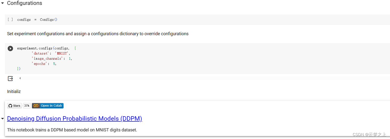
    # Set configurations. You can override the defaults by passing the values in the dictionary.
    experiment.configs(configs, {
        'dataset': 'CelebA',  # 'MNIST'
        'image_channels': 3,  # 1,
        'epochs': 100,  # 5,
    })

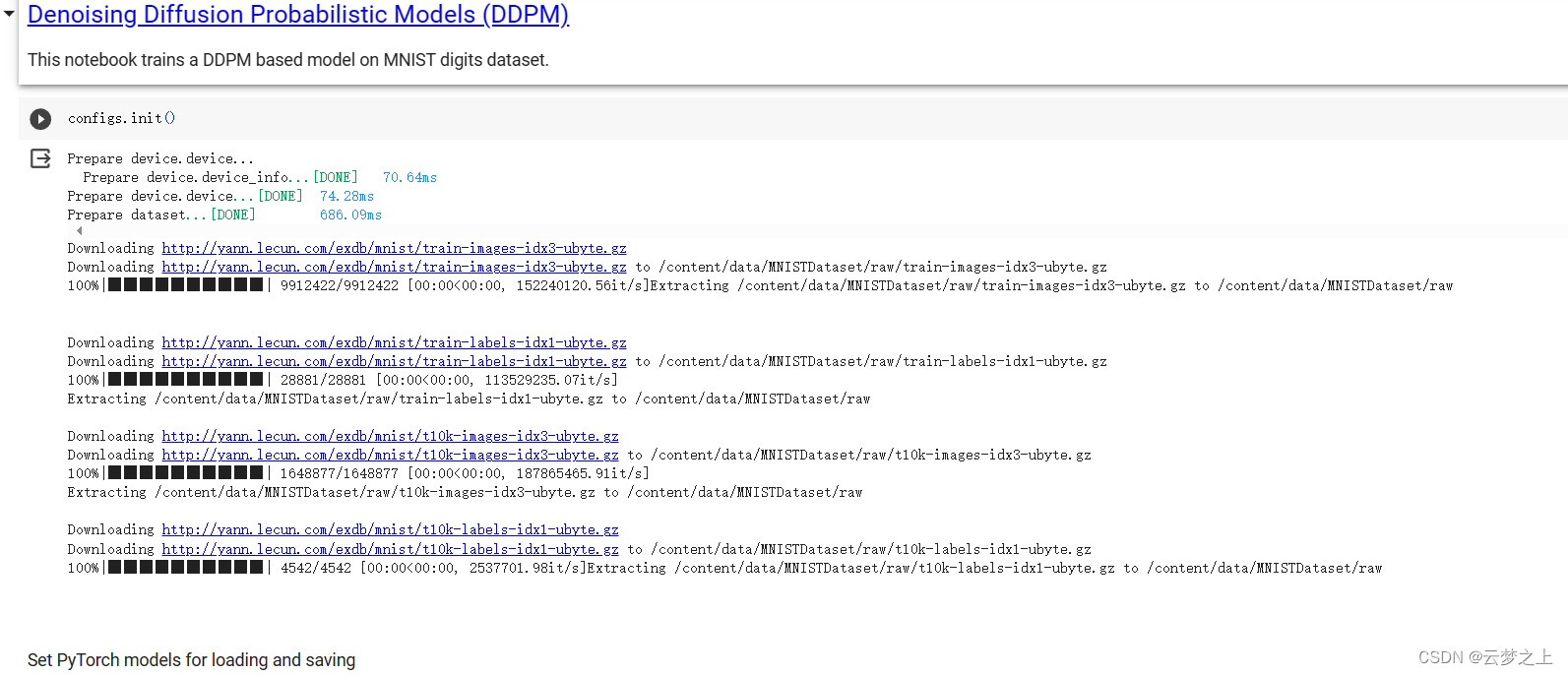
    # Initialize
    configs.init()

    # Set models for saving and loading
    experiment.add_pytorch_models({'eps_model': configs.eps_model})

    # Start and run the training loop
    with experiment.start():
        configs.run()



#
if __name__ == '__main__':
    main()

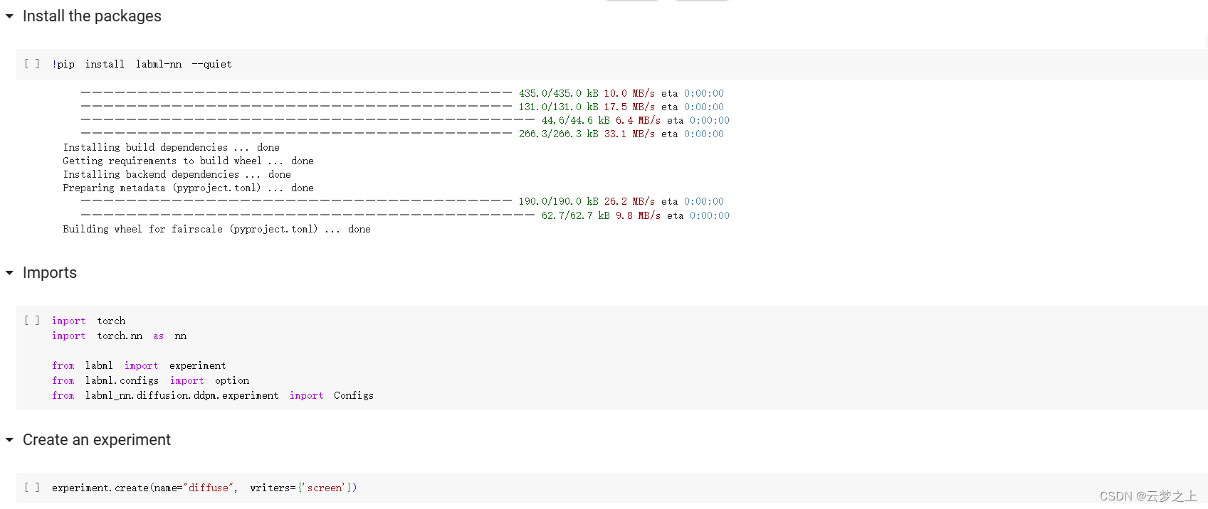
2.2.4 运行结果的展示

这里是部署在google的colab中运行的
具体部署的流程可以参考：
Colab 实用教程

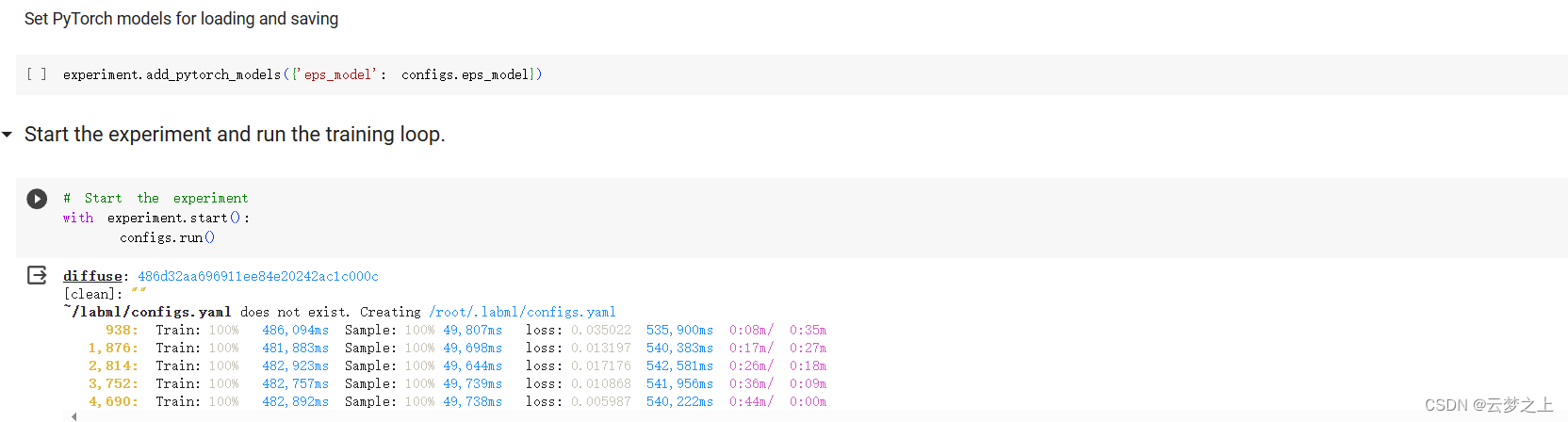
可以看取样生成的图片效果还是不错的