压制式干扰对脉冲雷达的干扰性能研究【附MATLAB代码】

干扰效果的研究能够为后续干扰工作打下基础，有效的评估干扰能力十分重要，本文研究了压制式干扰中射频噪声干扰、噪声调幅干扰、噪声调频干扰。对三种类型的压制式干扰进行性能研究，以脉冲雷达模型为干扰对象，采用信号处理方法探究三种压制式干扰对脉冲雷达目标回波的干扰效果。

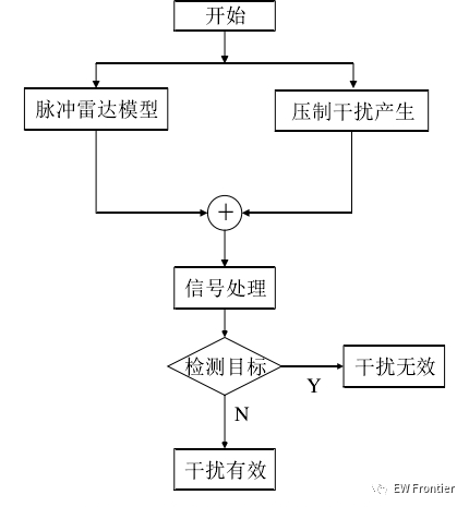
下图为探究压制式干扰性能的设计流程。脉冲雷达模型作为干扰对象，产生目标回波脉冲信号，压制式干扰模块产生射频噪声干扰、噪声调幅干扰、噪声调频干扰干扰信号，改变噪声干扰的功率并加载到脉冲雷达回波信号中以此模拟压制干扰影响下的雷达目标回波，此时雷达接收机接收到的回波信号中包含一定功率的噪声干扰。雷达接收机对接收到的总的回波进行信号处理，采用的信号处理方法包括脉冲压缩、动目标检测等。若经过信号处理后无法检测出目标，即该干扰信号对脉冲雷达的干扰性能有效，若经过信号处理后仍然能检测到目标，即该干扰信号无效。 是否检测到目标通过脉冲压缩后的图像进行评判。

低干信比：

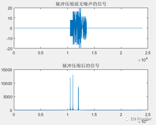
无噪声环境下脉冲压缩

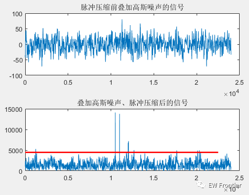
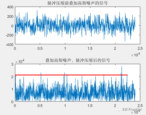
射频噪声干扰性能研究

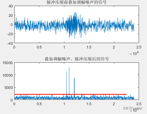
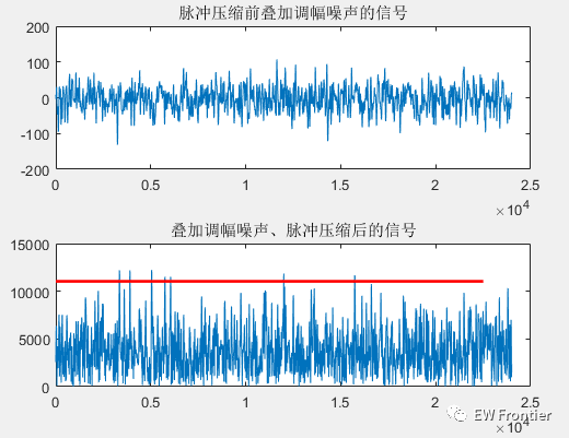
调幅噪声干扰脉冲压缩

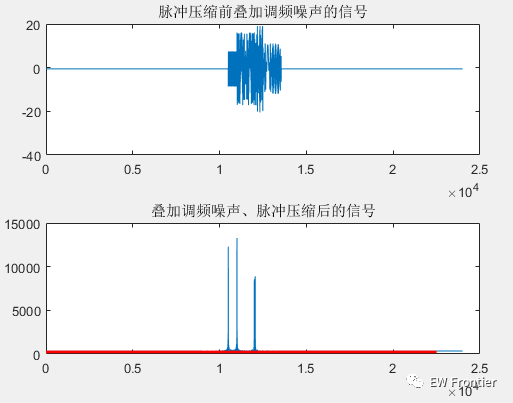
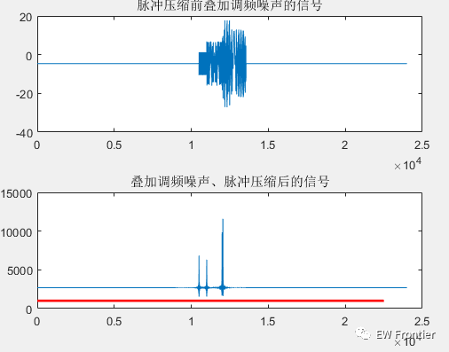
噪声调频干扰脉冲压缩

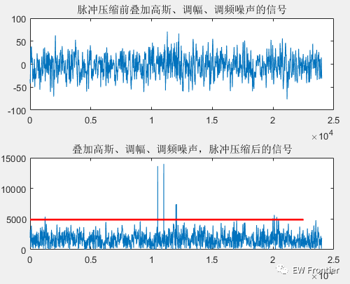
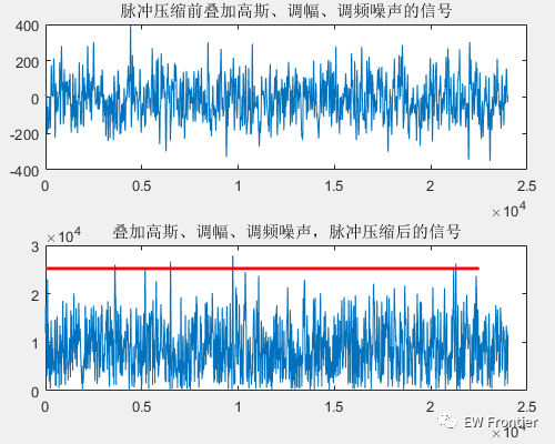
三种干扰叠加脉冲压缩

高干信比：

射频噪声干扰

调幅噪声干扰

调频噪声干扰

三种干扰叠加干扰

MATLAB代码

clc;
clear all;
close all;
​
%%
%雷达参数
c = 3e8;
A = 1;
tp = 10e-6;               %脉宽
B = 3e7;
fc = 0;
R_t = [10.5e3 11e3 12e3 (12e3)+50 13e3 (13e3)+20];
k = B/tp;                 %带宽和脉宽%%%线性调频信号的调频斜率
fs = 5*B;                 %抽样频率
PRF = 2000;               %脉冲重复频率
Tmax = 15*tp;             %雷达观察的距离时间范围
t = 0:1/fs:Tmax+tp;       %离散的时间采样
lamda = c/fs;
N = ceil((Tmax+tp)*fs);
​
%% 
%目标参数
N_target = 4;                  %目标个数
RCS_t = 5*rand(1,N_target)+5;  %随机生成目标的RCS，最大为10，最小为5
​
%% 
%回波模拟
[noise_nor,noise_nor_sum] = gsfb_tm(0,1,N,N_target);
​
noise_Am = noise_Am_tm(A,N,N_target);
noise_Fm = noise_Fm_tm(2*A,100,N,N_target);
temp  = 0;
for n_t = 1:N_target
    de = 2*R_t(n_t)/c;   %目标延时
    st = RCS_t(n_t)*rectpuls(t-de-tp/2,tp).*exp(-1i*pi*k*(t-de-tp/2).^2); %目标回波
    temp = temp+st;      %多个目标回波的叠加
end
y0 = temp;
y1 = temp+5*noise_nor_sum;
y2 = temp+5*noise_Am;
y3 = temp+5*noise_Fm;
y4 = temp+5*noise_nor_sum+5*noise_Am+5*noise_Fm;
​
%% 
%无噪声信号脉冲压缩
replica = A*rectpuls(t-tp/2,tp).*exp(-1i*pi*(B/tp).*(t-tp/2).^2);  %基带线性调频信号
nfft = length(t);
rfft0 = fft(replica,nfft); 
yfft0 = fft(y0,nfft);  
out0 = abs(ifft((conj(rfft0) .* (yfft0)))); 
pow = sum(out0.^2)/Tmax; %中频功率
% pow = sum(out0.^2)/(length(out0)*Tmax); %中频功率
​
%%
%有噪声信号的脉冲压缩
yfft1 = fft(y1,nfft);  
out1 = abs(ifft((conj(rfft0) .* (yfft1)))); 
noise_lv1 = out1-out0;
yfft2 = fft(y2,nfft);  
out2 = abs(ifft((conj(rfft0) .* (yfft2)))); 
noise_lv2 = out2-out0;
yfft3 = fft(y3,nfft);  
out3 = abs(ifft((conj(rfft0) .* (yfft3)))); 
noise_lv3 = out3-out0;
yfft4 = fft(y4,nfft);  
out4 = abs(ifft((conj(rfft0) .* (yfft4)))); 
noise_lv4 = out4-out0;
​
%%
%对发现概率的影响
Pfa = log(1e-6);
ut = zeros(1,4);
ut(1) = sqrt(-2*var(noise_lv1)*Pfa);%匹配滤波后的门限电压
ut(2) = sqrt(-2*var(noise_lv2)*Pfa);%匹配滤波后的门限电压
ut(3) = sqrt(-2*var(noise_lv3)*Pfa);%匹配滤波后的门限电压
ut(4) = sqrt(-2*var(noise_lv4)*Pfa);%匹配滤波后的门限电压
Y = zeros(1,4);
Y(1) = sum(abs(fft(out1,N)).^2)/N;
Y(2) = sum(abs(fft(out2,N)).^2)/N;
Y(3) = sum(abs(fft(out3,N)).^2)/N;
Y(4) = sum(abs(fft(out4,N)).^2)/N;
W = zeros(1,4);
W(1) = sum(abs(fft(noise_nor_sum)).^2)/N;
W(2) = sum(abs(fft(noise_Am)).^2)/N;
W(3) = sum(abs(fft(noise_Fm)).^2)/N;
W(4) = sum(abs(fft(noise_nor_sum+noise_Am+noise_Fm)).^2)/N;
a = zeros(1,4);
Pd = a;
for i = 1:4
    a(i) = 1e4*pow/W(i);
    x = normrnd(0,1,[1 1000]);
    y = normrnd(a(i),1,[1 1000]);
    Pdr = sqrt(x.^2+y.^2);
    Pd(i) = sum(Pdr>ut(i))/N;
end
​
%%
%压制系数
Ka = zeros(1,4);
for i = 1:4
    Ka(i) = W(i)/Y(i);
end
%%
%画图
figure,
subplot(2,1,1);plot(t*c/2,y0);title('脉冲压缩前无噪声的信号');
subplot(2,1,2);plot(c/2*t,out0);title('脉冲压缩后的信号');
%脉冲压缩后能看到4根谱线是因为R_t = [10.5e3 11e3 12e3 (12e3)+5 13e3 (13e3)+2]，
% 其中目标3与目标4、目标5与目标6距离过近，脉冲压缩后仍无法分辨
​
figure,
subplot(2,1,1);plot(t*c/2,y1);title('脉冲压缩前叠加高斯噪声的信号');
subplot(2,1,2);plot(c/2*t,out1);line([0,c/2*Tmax],[ut(1),ut(1)],'color','r','linewidth',2);
title('叠加高斯噪声、脉冲压缩后的信号');
​
figure,
subplot(2,1,1);plot(t*c/2,y2);title('脉冲压缩前叠加调幅噪声的信号');
subplot(2,1,2);plot(c/2*t,out2);line([0,c/2*Tmax],[ut(2),ut(2)],'color','r','linewidth',2);
title('叠加调幅噪声、脉冲压缩后的信号');
​
figure,
subplot(2,1,1);plot(t*c/2,y3);title('脉冲压缩前叠加调频噪声的信号');
subplot(2,1,2);plot(c/2*t,out3);line([0,c/2*Tmax],[ut(3),ut(3)],'color','r','linewidth',2);
title('叠加调频噪声、脉冲压缩后的信号');
​
figure,
subplot(2,1,1);plot(t*c/2,y4);title('脉冲压缩前叠加高斯、调幅、调频噪声的信号');
subplot(2,1,2);plot(c/2*t,out4);line([0,c/2*Tmax],[ut(4),ut(4)],'color','r','linewidth',2);
title('叠加高斯、调幅、调频噪声，脉冲压缩后的信号');