【限免】雷达目标生成与探测研究项目【附MATLAB代码】

最新推荐文章于 2024-06-26 13:58:35 发布

EW Frontier

最新推荐文章于 2024-06-26 13:58:35 发布

阅读量635

点赞数 16

文章标签： matlab 开发语言

本文链接：https://blog.csdn.net/m0_54016576/article/details/138389251

版权

文章来源：微信公众号：EW Frontier

课题背景

该项目的目标是模拟FMCW雷达检测运动目标，然后执行信号处理功能，以估计模拟目标的距离和多普勒速度。

图1：雷达模拟和检测的项目工作流程

FMCW波形设计

根据系统要求设计了一种调频连续波雷达波形。求啁啾带宽、时间和斜率。

图2：FMCW雷达系统需求设计规范

基于雷达规范，线性调频脉冲参数的值为：

·带宽：1.5e8 ·时间：7.3333e-06 ·斜率：2.0455e+13

仿真流程

模拟目标运动并计算每个时间戳的节拍或混合信号。应生成差拍信号，以便一旦实现距离FFT，它就给出正确的距离，即分配有+/- 10米误差容限的目标的初始位置。

对于移动目标模拟，尝试了2种不同的距离和相对速度设置。在第一个实验中，我使用了110米的初始目标范围和20米每秒的相对接近速度。我还试验了一个距离100米的目标，相对接近速度为每秒-40米。为了这个简单的研究，假设目标的速度在观察期间是恒定的。请注意，我没有向任何信号添加统计噪声。

图3：模拟目标的两个周期（共128个），初始距离为110米，接近速度为20米/秒

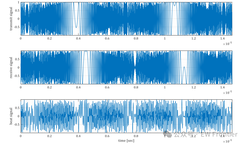
图4：模拟目标的两个周期（共128个），初始距离为100米，接近速度为-40米/秒

距离FFT

在差拍或混合信号上执行范围FFT并绘制结果。正确的实现应该在正确的范围内生成峰值，即分配目标的初始位置，误差容限为+/-10米。

图5：初始距离为110 m，相对速度为20 m/s时模拟目标的FFT

图6：初始距离为100 m，相对速度为-40 m/s时模拟目标的FFT

2D恒虚警概率

在距离多普勒图上实现二维恒虚警处理。二维恒虚警处理应能抑制噪声，分离出目标信号。

对于初始距离为110米、相对速度为20米/秒的模拟目标：

图7：阈值处理前的距离多普勒图

图8：基于CFAR的阈值处理后的距离多普勒图

下面是上一页中相同图像的目标的详细说明：

图9：阈值处理前距离多普勒图上目标放大图像

图10：阈值化后距离多普勒图上目标的放大图像

对于初始距离为100米和相对速度为-40米/秒的模拟目标：

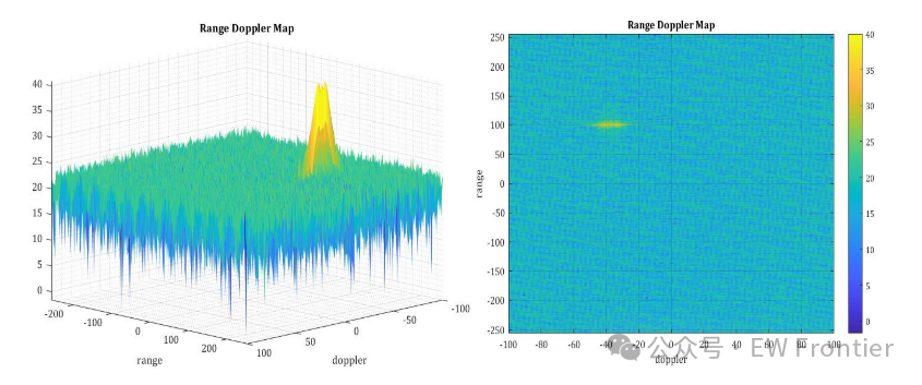
图11：阈值处理前的距离多普勒图

图12：基于CFAR的阈值处理后的距离多普勒图

下面是上一页中相同图像的目标的详细说明：

图13：阈值处理前距离多普勒图上目标的放大图像

图14：阈值化后距离多普勒图上目标的放大图像

CFAR

请简要说明以下内容：

2D CFAR过程的实施步骤

2D CFAR过程的训练单元、保护单元和偏移的选择

2D CFAR过程的实施步骤2D C

对距离多普勒图执行二维CFAR处理，该距离多普勒图是通过对每个线性调频脉冲中的差拍信号进行FFT以确定随时间的目标距离，然后对随时间的距离FFT进行第二FFT以确定跨越线性调频脉冲的相位变化率而生成的。因此，距离多普勒图表示我们对目标距离与多普勒速度随时间的估计。

图15：生成距离多普勒图

二维恒虚警处理是一种动态阈值方法，用于在杂波背景下检测目标。该阈值是通过估计周围箱中的噪声水平并乘以偏移量来计算的。其思想是根据估计的噪声水平自适应地改变阈值，以保持恒定的虚警率，该虚警率独立于杂波并包括真实目标。将阈值与仓的距离多普勒值进行比较，以确定是否存在目标。使用滑动窗口方法对距离多普勒图中的所有仓（减去外边界）重复该过程。

滑动窗由三部分组成。我们将每个正在评估的bin称为待测单元（CUT）。围绕CUT的是一个我们称之为保护单元的区域，它用于允许目标能量穿过距离多普勒图中的多个仓。这是必要的，以避免在下一步中破坏本地噪声水平估计。然后，我们通过计算CUT和保护单元周围的局部环形区域中的箱的样本平均值来生成局部噪声水平的估计值-这些被称为训练单元。一个小细节：在计算样本平均值之前，需要将训练小区值从对数dB转换为线性功率，然后转换回dB，以便将阈值与CUT中的距离多普勒值进行比较。这些参数的最佳值是应用/问题特定的。在这个项目中，我通过查看距离多普勒图中的二维目标范围，逐个手动调整了保护单元的数量和训练单元的数量：

图16：对于初始距离为110 m、接近速度为20 m/s的目标，选择以下窗口参数：距离维度（Gr）中的5个保护单元，多普勒维度（Gd）中的23个保护单元，距离维度（Tr）中的20个训练单元，以及多普勒维度（Td）中的10个训练单元。

接下来，将偏移项（我称之为"阈值噪声比"（tnr））添加到log dB空间中的估计噪声水平，以产生检测阈值。然后，我们将CUT中的信号与该阈值进行比较。如果CUT中的信号低于此阈值，我们将其设置为零，从而在距离多普勒图中对其进行抑制。如果CUT中的信号上升到阈值以上，我将保持该值不变（注意：项目步骤建议将其设置为1，但我更喜欢查看目标分布）。

对于偏移量的选择，我使用了一个试错过程，该过程包括可视化多个偏移量值的CFAR检测结果，然后选择一个最大化真实目标检测同时最小化错误检测数量的值。对于接近速度为20 m/s的110 m目标，以及相应的防护和训练单元参数，我选择偏移量为10。110 m目标偏移量参数扫描的恒虚警率检测结果如下所示：

图17：110 m目标在-20 m/s接近速度下，基于多个偏移量的CFAR检测结果

对于接近速度为-40 m/s的100 m目标，在距离维选择6个保护单元，在多普勒维选择22个保护单元，在距离维选择20个训练单元，在多普勒维选择10个训练单元，阈值偏移为9.0。这产生了上一节中看到的结果。

我必须考虑的另一个权衡是窗口大小与距离多普勒图中该窗口所施加的有效视场之间的反比关系。如果所选窗口尺寸过大，则可能会错过靠近边缘的目标。另一方面，太少的训练单元可能产生局部噪声水平的次优估计，并且太少的保护单元可能使目标信号泄漏到训练单元中，破坏噪声估计。因此，在评估车辆的整体传感器覆盖范围（检测范围与视场）时，应考虑窗口大小。

距离多普勒图外边界的单元必须根据滑动窗口的大小进行抑制。当在测试下的小区上循环时，我们通过跳过沿着最大和最小范围维度的Gr + Tr仓以及沿着最大和最小多普勒维度的Gd + Td仓来对此进行解释。然后，将CFAR处理的减小尺寸的输出映射回其在零阵列中的原始位置，该零阵列在尺寸上等同于全距离多普勒图：

图18：抑制距离多普勒图边界上的非阈值单元

MATLAB代码

maximumRange.m

% Constant False Alarm Rate
clear all; close all;

N = 1000; % Number of Samples
signal = abs(randn(N,1)); % Generate Random Noise

% Set Target Locations:
% Assign Targets to Bins 100, 200, 300 and 700
% Assign Target Amplitudes: 8, 9, 4, 11
signal([100 200 300 700]) = [8 9 4 11];
%signal([100 200 350 700]) = [8 15 7 13];

figure; plot(signal);

T = 12; % Number of Training Cells
G = 4; % Number of Guard Cells
tnr = 3.5; % define threshold-to-noise ratio
threshold_cfar = []; % define vector for threshold values
signal_cfar = []; % define vector for thresholded signal result

% Sliding window filter: make sure we give enough room at the end for the
% number of guard cells and training cells
for winIdx = 1:(N-(G+T))
    
    % Estimate the average noise across the training cells
    noise = sum(signal(winIdx:winIdx+T-1))/T; 
    
    % Compute threshold
    threshold = noise*tnr;
    threshold_cfar = [threshold_cfar,{threshold}];
    
    % Measure signal within the cell under test (CUT)
    CUTsig = signal(winIdx+T+G); % define as T+G cells away from the first training cell
    
    % If the signal level at CUT is below the threshold
    if CUTsig < threshold
        % then assign it a 0 value
        CUTsig = 0;
    end
    
    signal_cfar = [signal_cfar, {CUTsig}];
end

% Plot the filtered signal
figure;
plot(cell2mat(signal_cfar),'g--');

figure; plot(signal);
hold on; plot(cell2mat(circshift(threshold_cfar,G)),'r--','LineWidth',2);
hold on; plot(cell2mat(circshift(signal_cfar,(T+G))),'g.','MarkerSize',14);
legend('Signal','CFAR Threshold','Detection');

% 2-D CFAR on Range-Doppler Map
% 1. Determine the number of Training Cells (Tr & Td) and the number of
% Guard Cells (Gr & Gd) for each dimension 
% 2. Slide the Cell Under Test (CUT) across the complete cell matrix
% 3. Select the grid that includes the training, guard and test cells. Grid
% Size = (2Tr+2Gr+1)(2Td+2Gd+1) 
% 4. The total number of cells in the guard region and cell under test.
% (2Gr+1)(2Gd+1) 
% 5. This gives the Training Cells : (2Tr+2Gr+1)(2Td+2Gd+1) - (2Gr+1)(2Gd+1)
% 6. Measure and average the noise across all the training cells. This
% gives the threshold 
% 7. Add the offset (if in signal strength in dB) to the threshold to keep
% the false alarm to the minimum 
% 8. Determine the signal level at the Cell Under Test 
% 9. If the CUT signal level is greater than the Threshold, assign a value
% of 1, else equate it to zero 
% 10. Since the cell under test are not located at the edges, due to the
% training cells occupying the edges, we suppress the edges to zero. Any
% cell value that is neither 1 nor a 0, assign it a zero  
% 
% *************************************************************************
% 2-D FFT

% Create and plot 2-D data with repeated blocks
P = peaks(20);
X = repmat(P,[5 10]);
figure
imagesc(X);

% Compute the 2-D Fourier Transform of the data
X_fft = fft2(X);

% Shift the zero-frequency component to the center of the output
X_fft = abs(fftshift(X_fft));

% Plot the resulting 100-by-200 matrix, which is the same size as X
figure; imagesc(log(X_fft));

% *************************************************************************
% Find the frequency components of a signal buried in noise

% Define FFT parameters
fs = 1.0e3; % sampling frequency
T = 1/fs; % sampling period
L = 1500; % length of signal (time duration) in ms
%N = 1024; % number of samples

% Define a signal and add noise
t = (0:L-1)*T; % time vector
f = [77 43]; % frequency of two signals in Hz
A = [0.7 2.0]; % signal amplitudes
%S = 0.7*sin(2*pi*77*t) + 2*sin(2*pi*43*t); % note: class notes suggested cos
signal = sum(A'.*sin(2*pi*f'.*t));
noisedSignal = signal; % + 2*randn(size(t));

figure; plot(1000*t(1:50),noisedSignal(1:50));
title('Signal Plus Zero-Mean Random Noise');
xlabel('time [ms]');
ylabel('noised signal');

% Compute the FFT of the noised signal
signal_fft = fft(noisedSignal); %,N);

% Compute the amplitude of the normalized signal
%signal_fft = abs(signal_fft);  % take the magnitude of the fft
signal_fft = abs(signal_fft/L); % take the amplitude of the fft

% Compute the single-sided spectrum based on the even-valued signal length L
%signal_fft = signal_fft(1:L/2-1); % discard negative half of fft (mirrored image)
signal_fft = signal_fft(1:L/2+1); % discard negative half of fft (mirrored image)

freq = fs*(0:(L/2))/L;
figure; plot(freq,signal_fft);
title('Single-Sided Amplitude Spectrum of Noisy Signal');
xlabel('frequency [Hz]');
ylabel('amplitude');

% *************************************************************************
% Doppler Velocity Calculation
% Calculate the velocity in m/s of four targets with the following Doppler
% frequency shifts: [3 KHz, -4.5 KHz, 11 KHz, -3 KHz]

% Radar Operating Frequency (Hz)
fc = 77.0e9;

% Speed of Light (meters/sec)
c = 3*10^8;

% Wavelength
lambda = c/fc;

% Doppler Shifts in Hz
fd = [3.0e3, -4.5e3, 11.0e3, -3e3];

% Velocity of the targets
%fd = (2*vr)/lambda;
vr = (fd*lambda)/2;

disp(vr)

% velocity = distance/time

% *************************************************************************
% Given the radar maximum range of 300m and range resolution of 1m,
% calculate the range of four targets with the following measured beat
% frequencies: 0MHz, 1.1MHz, 13MHz, 24MHz

% Speed of Light (meters/sec)
c = 3*10^8;

% Maximum Detectable Range in Meters
Rmax = 300;

% Range Resolution in Meters
deltaR = 1;

% Bsweep of Chirp
Bsweep = c/2*deltaR;

% The sweep/chirp time can be computed based on the time needed for the signal to
% travel the maximum range. In general, for an FMCW radar system, the sweep
% time should be at least 5 to 6 times the round trip time. This example
% uses a factor of 5.5:
Tchirp = 5.5*(Rmax*2/c); % 5.5 times the trip time at maximum range

% Beat Frequencies (Hz) of four targets:
fb = [0e6,1.1e6,13e6,24e6];

% Range for every target (meters)
calculated_range = c*Tchirp*fb/(2*Bsweep); 

disp(calculated_range);

% *************************************************************************
% Operating Frequency (Hz)
fc = 77.0e9;
% Wavelength
lambda = c/fc;
% Transmitted Power (W)
Pt = 3e-3;

% Antenna Gain (linear)
G = 10000;

% Minimum Detectable Power
Ps = 1e-10;

% RCS of a car
RCS = 100;

Range = (((10*log10(Pt*1000))*(G^2)*(lambda^2)*RCS)/(Ps*((4*pi)^3)))^(1/4);
disp(Range);

radarTargetGenerationAndDetection.m

% +---------------------------------------+
% |  Radar Target Generation & Detection  |                                 
% |  Jasmine Taketa-Tran, 5 October 2020  |
% +---------------------------------------+
clear all; close all;

%% Define Radar Specifications
% Configure the FMCW Waveform based on the System Requirements

fc= 77.0e9; % Operating Carrier Frequency (Hz)
c = 3.0e8; % Speed of Light (meters/sec)
lambda = c/fc; % Wavelength
Rmax = 200; % Maximum Detectable Range (meters)
Vmax = 70; % Maximum Velocity (meters/sec)
deltaR = 1.0; % Range Resolution in (meters)
deltaV = 3.0; % Velocity Resolution (meters/sec)

%% Compute FMCW Waveform Parameters
% Calculate the FMCW waveform parameters given the requirements specs

% Bandwidth of each chirp at the given range resolution:
Bsweep = c/(2*deltaR);

% Sweep Time for each chirp defined at 5.5x round trip time at max range:
Tsweep = 5.5*(Rmax*2/c);

% Slope of the chirp
Slope = Bsweep/Tsweep;

% The number of chirps in one sequence
Nd = 128; % #of doppler cells OR #of sent periods

% The number of samples on each chirp
Nr = 1024; % for length of time OR # of range cells


%% Model Signal Propagation for the Moving Target Simulation

% Set initial range and velocity of the target
targetRange = 110; %100; % Initial Distance to the Target (<= 200 m)
targetVelocity = 20; %-40; % Closing Velocity of Target (-70 to +70 m/s)

% Initialize vectors to store variable time histories
time = linspace(0,Nd*Tsweep,Nr*Nd); % time vector
Tx = zeros(1,length(time)); % transmit signal
Rx = zeros(1,length(time)); % receive signal
beatSig = zeros(1,length(time)); % beat frequency
range2Tgt = zeros(1,length(time)); % range to target
tau = zeros(1,length(time)); % time delay (trip time for the signal)

for tIdx = 1:length(time)
    
    % Displace the target based on the assumption of constant velocity
    range2Tgt(tIdx) = targetRange + (targetVelocity * time(tIdx));
    
    % Ensure that the targetRange does not exceed the maximum detectable
    % range of the radar. If it does, then flag it as undetectable.
    if range2Tgt(tIdx) > Rmax
        range2Tgt(tIdx) = NaN;
    end
    
    % Update the trip/delay time for the received signal
    tau(tIdx) = (range2Tgt(tIdx)*2)/c;
    
    % For each time stamp, update the transmit and receive signals
    % Receive signal is the time-delayed version of the transmit signal
    Tx(tIdx) = cos(2*pi*((fc*time(tIdx)) + ((Slope*(time(tIdx)^2))/2)));
    Rx(tIdx) = cos(2*pi*((fc*(time(tIdx)-tau(tIdx))) +...
        ((Slope*((time(tIdx)-tau(tIdx))^2))/2)));
end

% % Add 20% random noise to the signals
% Tx = Tx.*(1 + 0.2*randn(size(time)));
% Rx = Rx.*(1 + 0.2*randn(size(time)));

% For each displacement, determine the beat signal (frequency shift)
beatSig = Tx.*Rx; 

figure; subplot(3,1,1); plot(time(1:(Nr*2)),Tx(1:(Nr*2))); ylabel('transmit signal'); axis tight; grid on; grid minor; set(gca,'FontName','Cambria');
subplot(3,1,2); plot(time(1:(Nr*2)),Rx(1:(Nr*2))); ylabel('receive signal'); axis tight; grid on; grid minor; set(gca,'FontName','Cambria');
subplot(3,1,3); plot(time(1:(Nr*2)),beatSig(1:(Nr*2))); ylabel('beat signal'); axis tight; xlabel('time [sec]'); grid on; grid minor; set(gca,'FontName','Cambria');
subplot(3,1,1); hold on; title(sprintf('un-noised signal across 2 chirps on a target at initial range of %dm & %d m/s closing velocity',targetRange,targetVelocity));


%% Estimate the Range to Target
% Perform 1D FFT on the beat signal to estimate the range to target

% Reshape the mix signal into number of range samples (Nr) 
% and number of doppler samples (Nd) to form an Nr-by-Nd array
% Nr and Nd will also be used for the FFT sizes
beatMat = reshape(beatSig,[Nr Nd]);
range2TgtMat = reshape(range2Tgt,[Nr Nd]);

% Compute the normalized FFT of the beat signal along the range dimension
beat_fft = fft(beatMat,Nr)/Nr;

% Compute the amplitude of the normalized signal
beat_fft = abs(beat_fft);

% Compute the single-sided spectrum based on the even-valued signal length
beat_fft = beat_fft(1:Nr/2+1,:); % discard negative half of fft

figure('Name','Range from First FFT'); plot(beat_fft);
title('Amplitude Spectrum of the Beat Signal');
xlabel('range [m]'); ylabel('amplitude'); grid on; grid minor;
set(gca,'FontName','Cambria'); axis tight;
xticks(1:50:513); xticklabels(0:50:512);


%% Generate the Range Doppler Map (RDM)
% Perform a 2D FFT on the beat signal to generate a Range Doppler Map
% Perform CFAR processing on the output of the 2nd FFT to find the target
beatMat = reshape(beatSig,[Nr Nd]);

% 2D FFT using the FFT size for both dimensions
sig_fft2 = fft2(beatMat,Nr,Nd);

% Take just one side of signal in the range dimension
sig_fft2 = sig_fft2(1:Nr/2,1:Nd);
sig_fft2 = fftshift(sig_fft2);
RDM = abs(sig_fft2);
RDM = 10*log10(RDM);

% Plot the output of 2D FFT as a function of range and velocity
doppler_axis = linspace(-100,100,Nd);
range_axis = linspace(-200,200,Nr/2)*((Nr/2)/400);

figure; surf(doppler_axis,range_axis,RDM);
xlabel('doppler'); ylabel('range'); 
title('Range Doppler Map');
set(gca,'FontName','Cambria');
grid on; grid minor; axis tight;

figure; contourf(doppler_axis,range_axis,RDM);
xlabel('doppler'); ylabel('range'); 
title('Range Doppler Map');
set(gca,'FontName','Cambria'); colorbar;
grid on; grid minor;


%% Perform CFAR Thresholding on the RDM to Detect the Target
% Note: For a Target at 100m, Gr = 6, Gd = 22 & tnr = 9
%       For a Target at 110m, Gr = 5, Gd = 23 & tnr = 10

% Select the Number of Training Cells
Tr = 20; % Number of Training Cells in the Range Dimension
Td = 10; % Number of Training Cells in the Doppler Dimension

% Select the Number of Guard Cells
Gr = 5;  % Number of Guard Cells in the Range Dimension
Gd = 23; % Number of Guard Cells in the Doppler Dimension

% Offset the threshold by SNR value in dB
tnr = 10; % Define the Threshold-to-Noise Ratio

% Slide the window filter across the Range Doppler Map
% Allow an outer image buffer for Guard & Training cells
for i = Tr+Gr+1:(Nr/2)-(Gr+Tr)
    for j = Td+Gd+1:Nd-(Gd+Td)
        
        % Step through the bins & grid surrounding the Cell Under Test
        noise_level = zeros(1,1);
        for p = i-(Tr+Gr):i+Tr+Gr
            for q = j-(Td+Gd):j+Td+Gd
                
                % Exclude the Guard Cells and the Cell Under Test
                if (abs(i-p)>Gr) || (abs(j-q)>Gd)
                    
                    % Convert the logarithmic dB value to linear power
                    % Then sum the noise across the Training Cells
                    noise_level = noise_level + db2pow(RDM(p,q));
                end
            end
        end
        
        % Compute threshold based on the noise and offset (tnr)
        numGridCells = ((2*Tr)+(2*Gr)+1)*((2*Td)+(2*Gd)+1);
        numGuardCells = Gr*Gd;
        numTrainCells = numGridCells - numGuardCells - 1;
        
        % Estimate the average noise across the Training Cells
        % Convert back to logarithmic dB after obtaining the average
        threshold = pow2db(noise_level/numTrainCells);
        threshold = threshold + tnr; % multiplying in linear space
        
        % Compare the Cell Under Test to the Detection Threshold
        CUT = RDM(i,j); % get signal within the Cell Under Test
        if CUT < threshold % if it is below threshold
            RDM(i,j) = 0; % then assign it a value of 0
%       else % if it is above threshold
%           RDM(i,j) = 1; % then assign it a value of 1
        end    
    end
end

% Suppress edges of the Range Doppler Map to account for the presence 
% of Training and Guard Cells surrounding the Cell Under Test 
RDM_thresholded = zeros(size(RDM));
RDM_thresholded(Tr+Gr+1:(Nr/2)-(Gr+Tr),Td+Gd+1:Nd-(Gd+Td)) = ...
    RDM(Tr+Gr+1:(Nr/2)-(Gr+Tr),Td+Gd+1:Nd-(Gd+Td));

% Plot the filtered RDM as a function of range and velocity
figure; surf(doppler_axis,range_axis,RDM_thresholded);
title('Range Doppler Map after CFAR Thresholding');
xlabel('doppler'); ylabel('range'); axis tight;
set(gca,'FontName','Cambria'); grid on; grid minor;

figure; contourf(doppler_axis,range_axis,RDM_thresholded);
title('Range Doppler Map after CFAR Thresholding');
xlabel('doppler'); ylabel('range'); axis tight;
set(gca,'FontName','Cambria'); colorbar;
grid on; grid minor;

Sensor Fusion Using Synthetic Radar .m

clear all; close all;
%% Sensor Fusion Using Synthetic Radar 
%% Generate the Scenario
% Scenario generation comprises generating a road network, defining
% vehicles that move on the roads, and moving the vehicles.
% 
% Test the ability of the sensor fusion to track a
% vehicle that is passing on the left of the ego vehicle. The scenario
% simulates a highway setting, and additional vehicles are in front of and
% behind the ego vehicle.

% Define an empty scenario.
scenario = drivingScenario;
scenario.SampleTime = 0.01;

%% 
% Add a stretch of 500 meters of typical highway road with two lanes. The 
% road is defined using a set of points, where each point defines the center of 
% the road in 3-D space. 
roadCenters = [0 0; 50 0; 100 0; 250 20; 500 40];
%roadWidth = 7.2; % two lanes, each 3.6 meters wide
road(scenario, roadCenters, 'lanes', lanespec(2));
%road(scenario, roadCenters, roadWidth);

%% 
% Create the ego vehicle and three cars around it: one that overtakes the
% ego vehicle and passes it on the left, one that drives right in front of
% the ego vehicle and one that drives right behind the ego vehicle. All of
% the cars follow the trajectory defined by the road waypoints by using the
% path driving policy. The passing car will start on the right lane, move
% to the left lane to pass, and return to the right lane.

% Create the ego vehicle that travels at 25 m/s along the road.  Place the
% vehicle on the right lane by subtracting off half a lane width (1.8 m)
% from the centerline of the road. Note: Class notes use call to "path"
% function instead of "trajectory" function.
egoCar = vehicle(scenario, 'ClassID', 1);
trajectory(egoCar, roadCenters(2:end,:) - [0 1.8], 25); % in the right lane

% Add a car in front of the ego vehicle
leadCar = vehicle(scenario, 'ClassID', 1);
trajectory(leadCar, [70 0; roadCenters(3:end,:)] - [0 1.8], 25); % in the right lane

% Add a car that travels at 35 m/s along the road and passes the ego vehicle
passingCar = vehicle(scenario, 'ClassID', 1);
waypoints = [0 -1.8; 50 1.8; 100 1.8; 250 21.8; 400 32.2; 500 38.2];
trajectory(passingCar, waypoints, 35);

% Add a car behind the ego vehicle
chaseCar = vehicle(scenario, 'ClassID', 1);
trajectory(chaseCar, [25 0; roadCenters(2:end,:)] - [0 1.8], 25); % in the right lane

%% Define Radar Sensors
% Simulate an ego vehicle that has 6 radar sensors covering the entire 360
% degree field-of-view. The sensors have some overlap and some coverage
% gaps. The ego vehicle is equipped with a long-range radar sensor on both
% the front and the back of the vehicle. Each side of the vehicle has two
% short-range radar sensors, each covering 90 degrees. One sensor on each
% side covers from the middle of the vehicle to the back. The other sensor
% on each side covers from the middle of the vehicle forward. The figure in
% the next section shows the coverage.

sensors = cell(6,1);

% Front-facing long-range radar sensor at the center of the front bumper of the car.
sensors{1} = radarDetectionGenerator('SensorIndex', 1, 'Height', 0.2, 'MaxRange', 174, ... 
    'SensorLocation', [egoCar.Wheelbase + egoCar.FrontOverhang, 0], 'FieldOfView', [20, 5]);

% Rear-facing long-range radar sensor at the center of the rear bumper of the car.
sensors{2} = radarDetectionGenerator('SensorIndex', 2, 'Height', 0.2, 'Yaw', 180, ...
    'SensorLocation', [-egoCar.RearOverhang, 0], 'MaxRange', 174, 'FieldOfView', [20, 5]);

% Rear-left-facing short-range radar sensor at the left rear wheel well of the car.
sensors{3} = radarDetectionGenerator('SensorIndex', 3, 'Height', 0.2, 'Yaw', 120, ...
    'SensorLocation', [0, egoCar.Width/2], 'MaxRange', 30, 'ReferenceRange', 50, ...
    'FieldOfView', [90, 5], 'AzimuthResolution', 10, 'RangeResolution', 1.25);

% Rear-right-facing short-range radar sensor at the right rear wheel well of the car.
sensors{4} = radarDetectionGenerator('SensorIndex', 4, 'Height', 0.2, 'Yaw', -120, ...
    'SensorLocation', [0, -egoCar.Width/2], 'MaxRange', 30, 'ReferenceRange', 50, ...
    'FieldOfView', [90, 5], 'AzimuthResolution', 10, 'RangeResolution', 1.25);

% Front-left-facing short-range radar sensor at the left front wheel well of the car.
sensors{5} = radarDetectionGenerator('SensorIndex', 5, 'Height', 0.2, 'Yaw', 60, ...
    'SensorLocation', [egoCar.Wheelbase, egoCar.Width/2], 'MaxRange', 30, ...
    'ReferenceRange', 50, 'FieldOfView', [90, 5], 'AzimuthResolution', 10, ...
    'RangeResolution', 1.25);

% Front-right-facing short-range radar sensor at the right front wheel well of the car.
sensors{6} = radarDetectionGenerator('SensorIndex', 6, 'Height', 0.2, 'Yaw', -60, ...
    'SensorLocation', [egoCar.Wheelbase, -egoCar.Width/2], 'MaxRange', 30, ...
    'ReferenceRange', 50, 'FieldOfView', [90, 5], 'AzimuthResolution', 10, ...
    'RangeResolution', 1.25);


%% Create a Multi-Object Tracker
% Create a multi-object tracker to track the vehicles that are close to the
% ego vehicle. The tracker uses the initSimDemoFilter supporting function
% to initialize a constant velocity linear Kalman filter that works with
% position and velocity. 
% 
% Tracking is done in 2-D. Although the sensors return measurements in 3-D,
% the motion itself is confined to the horizontal plane, so there is no
% need to track the height.

%% TODO*
% Change the Tracker Parameters and explain the reasoning behind selecting
% the final values. You can find more about parameters here:
% https://www.mathworks.com/help/driving/ref/multiobjecttracker-system-object.html 
% Note: Kalman Filter is defined in initSimDemoFilter function further below
tracker = multiObjectTracker('FilterInitializationFcn', @initSimDemoFilter, ...
    'AssignmentThreshold', 30, 'ConfirmationParameters', [4 5], 'NumCoastingUpdates', 5);
positionSelector = [1 0 0 0; 0 0 1 0]; % Position selector
velocitySelector = [0 1 0 0; 0 0 0 1]; % Velocity selector

% Create the display and return a handle to the bird's-eye plot
BEP = createDemoDisplay(egoCar, sensors);


%% Simulate the Scenario
% The following loop moves the vehicles, calls the sensor simulation, and
% performs the tracking.
% 
% Note that the scenario generation and sensor simulation can have
% different time steps. Specifying different time steps for the scenario
% and the sensors enables you to decouple the scenario simulation from the
% sensor simulation. This is useful for modeling actor motion with high
% accuracy independently from the sensor'
s
 measurement rate.
% 
% Another example is when the sensors have different update rates. Suppose
% one sensor provides updates every 20 milliseconds and another sensor
% provides updates every 50 milliseconds. You can specify the scenario with
% an update rate of 10 milliseconds and the sensors will provide their
% updates at the correct time.
% 
% In this example, the scenario generation has a time step of 0.01 second,
% while the sensors detect every 0.1 second. The sensors return a logical
% flag (isValidTime) that is true if the sensors generated detections.
% This flag is used to call the tracker only when there are detections.
% 
% Another important note is that the sensors can simulate multiple
% detections per target, in particular when the targets are very close to
% the radar sensors. Because the tracker assumes a single detection per
% target from each sensor, you must cluster the detections before the
% tracker processes them. This is done by the function clusterDetections.
% See the 'Supporting Functions' section.

toSnap = true;
while advance(scenario) && ishghandle(BEP.Parent)    
    
    % Get the scenario time
    time = scenario.SimulationTime;
    
    % Get the position of the other vehicle in ego vehicle coordinates
    ta = targetPoses(egoCar);
    
    % Simulate the sensors
    detections = {};
    isValidTime = false(1,6);
    for i = 1:6
        [sensorDets,numValidDets,isValidTime(i)] = sensors{i}(ta, time);
        if numValidDets
            detections = [detections; sensorDets]; %#ok<AGROW>
        end
    end
    
    % Update the tracker if there are new detections from the sensors
    if any(isValidTime)
        
        vehicleLength = sensors{1}.ActorProfiles.Length;
        
        % Run the clustering function to generate detections
        detectionClusters = clusterDetections(detections, vehicleLength);
        
        % Update the confirmed tracks
        confirmedTracks = updateTracks(tracker, detectionClusters, time);
        
        % Update bird's-eye plot
        updateBEP(BEP, egoCar, detections, confirmedTracks, positionSelector, velocitySelector);
    end
    
    % Snap a figure for the document when the car passes the ego vehicle
    if ta(1).Position(1) > 0 && toSnap
        toSnap = false;
        snapnow
    end
end

%% Define the Kalman Filter
% Define the Kalman Filter here to be used with multiObjectTracker.
% In Matlab, a trackingKF function can be used to initiate a Kalman Filter
% for any type of Motion Model. This includes the 1D, 2D or 3D constant
% velocity or constant acceleration models.
% This function initializes a constant velocity filter based on a detection.
function filter = initSimDemoFilter(detection)

% Use a 2-D constant velocity model to initialize a trackingKF filter
% The state vector is [x;vx;y;vy], where x and y are 2D posiiton
% coordinates, and vx and vy are 2D velocity estimates
% The detection measurement vector is [x;y;vx;vy]
% The measurement model assumes that the actual measurement at any tiven
% time is related to the current state by: z = H*x
% As a result, the measurement model is H = [1 0 0 0; 0 0 1 0; 0 1 0 0; 0 0 0 1]

% Implement the Kalman filter using trackingKF function
H = [1 0 0 0; 0 0 1 0; 0 1 0 0; 0 0 0 1];

% Using this measurement model, the state can be derived from the
% measurements:
%    x = H'
*z;
%    state = H*detection.Measurement;
% Furthermore, the generated measurement noise and measurement model can be
% used to define the state covariance matrix:
%    stateCovariance = H'*detection.MeasurementNoise*H;

filter = trackingKF('
MotionModel
','
2
D Constant Velocity
',...
    '
State
', H'
*detection.Measurement,...
    'MeasurementModel', H,...
    'StateCovariance', H'*detection.MeasurementNoise*H,...
    '
MeasurementNoise
', detection.MeasurementNoise);
end

%% Cluster Detections
% This function merges multiple detections suspected to be of the same
% vehicle to a single detection. The function looks for detections that are
% closer than the size of a vehicle. Detections that fit this criterion are
% considered a cluster and are merged to a single detection at the centroid
% of the cluster. The measurement noise is modified to represent the
% possibility that each detection can be anywhere on the vehicle. As a
% result, the noise should have the same size as the vehicle size. In
% addition, this function removes the third dimension of the measurement
% (the height) and reduces the measurement vector to [x;y;vx;vy]. 
function detectionClusters = clusterDetections(detections, vehicleSize)

N = numel(detections);
distances = zeros(N);
% Loop over all possible pairs of detections
for i = 1:N
    for j = i+1:N
        % If the detections are from the same sensor
        if detections{i}.SensorIndex == detections{j}.SensorIndex
            % then record the Euclidean distance between them
            distances(i,j) = norm(detections{i}.Measurement(1:2) - detections{j}.Measurement(1:2));
        else
            distances(i,j) = inf;
        end
    end
end

leftToCheck = 1:N;
i = 0;
detectionClusters = cell(N,1);
% While the detection list is not empty and there are still detections to
% be grouped/clustered
while ~isempty(leftToCheck)    
    % Remove the detections that are in the same cluster as the one under consideration
    
    % Pick the first detection in the remaining check list
    underConsideration = leftToCheck(1);
    
    % Cluster detections with distances to the current pick that are within
    % the vehicle size. Group those detections and their respective radar
    % sensor measurements, including range and velocity measurements.
    clusterInds = (distances(underConsideration,leftToCheck) < vehicleSize);
    detInds = leftToCheck(clusterInds);
    clusterDets = [detections{detInds}];
    clusterMeas = [clusterDets.Measurement];
    
    % Take the mean range and velocity across the group
    meas = mean(clusterMeas,2);
    % Note: the radar measurement vector has 6 values, where range and
    % velocity for x and y coordinates reside at indices 1, 2, 4 and 5:
    % [x, y, -, Vx, Vy, -]
    meas2D = [meas(1:2); meas(4:5)];
    
    % Create a new cluster ID
    i = i + 1;
    % Assign the current group of detections to the same ID
    detectionClusters{i} = detections{detInds(1)};
    % Assign cluster range and velocity based on group member averages
    detectionClusters{i}.Measurement = meas2D;
    
    % Delete all detections belonging to the current group from the
    % remaining list of detections to cluster
    leftToCheck(clusterInds) = [];
    
    % Repeat in while loop until the detection list is empty
end
detectionClusters(i+1:end) = [];

% Since the detections are now for clusters, modify the noise to represent
% that they are of the whole car
for i = 1:numel(detectionClusters)
    measNoise(1:2,1:2) = vehicleSize^2 * eye(2);
    measNoise(3:4,3:4) = eye(2) * 100 * vehicleSize^2;
    detectionClusters{i}.MeasurementNoise = measNoise;
end
end


%% Create Demo Display
% This function creates a three-panel display:
% # Top-left corner of display: A top view that follows the ego vehicle.
% # Bottom-left corner of display: A chase-camera view that follows the ego vehicle.
% # Right-half of display: A <matlab:doc('
birdsEyePlot
') bird'
s
-eye plot> display.
function BEP = createDemoDisplay(egoCar, sensors)
    % Make a figure
    hFigure = figure('Position', [0, 0, 1200, 640], 'Name', 'Sensor Fusion with Synthetic Data Example');
    movegui(hFigure, [0 -1]); % Moves the figure to the left and a little down from the top    

    % Add a car plot that follows the ego vehicle from behind
    hCarViewPanel = uipanel(hFigure, 'Position', [0 0 0.5 0.5], 'Title', 'Chase Camera View');
    hCarPlot = axes(hCarViewPanel);
    chasePlot(egoCar, 'Parent', hCarPlot);

    % Add a car plot that follows the ego vehicle from a top view
    hTopViewPanel = uipanel(hFigure, 'Position', [0 0.5 0.5 0.5], 'Title', 'Top View');
    hCarPlot = axes(hTopViewPanel);
    chasePlot(egoCar, 'Parent', hCarPlot, 'ViewHeight', 130, 'ViewLocation', [0 0], 'ViewPitch', 90);
    
    % Add a panel for a bird's-eye plot
    hBEVPanel = uipanel(hFigure, '
Position
', [0.5 0 0.5 1], '
Title
', '
Bird
''
s
-Eye Plot
');
    
    % Create bird'
s
-eye plot 
for
 the ego car 
and
 sensor coverage
    hBEVPlot = axes(hBEVPanel);
    frontBackLim = 60;
    BEP = birdsEyePlot('Parent', hBEVPlot, 'Xlimits', [-frontBackLim frontBackLim], 'Ylimits', [-35 35]);
    
    % Plot the coverage areas for radars
    for i = 1:6
        cap = coverageAreaPlotter(BEP,'FaceColor','red','EdgeColor','red');
        plotCoverageArea(cap, sensors{i}.SensorLocation,...
            sensors{i}.MaxRange, sensors{i}.Yaw, sensors{i}.FieldOfView(1));
    end
    
    % Plot the coverage areas for vision sensors
%     for i = 7:8
%         cap = coverageAreaPlotter(BEP,'FaceColor','blue','EdgeColor','blue');
%         plotCoverageArea(cap, sensors{i}.SensorLocation,...
%             sensors{i}.MaxRange, sensors{i}.Yaw, 45);
%     end
    
    % Create a vision detection plotter put it in a struct for future use
%     detectionPlotter(BEP, 'DisplayName','vision', 'MarkerEdgeColor','blue', 'Marker','^');
    
    % Combine all radar detections into one entry and store it for later update
    detectionPlotter(BEP, 'DisplayName','radar', 'MarkerEdgeColor','red');
    
    % Add road borders to plot
    laneMarkingPlotter(BEP, 'DisplayName','lane markings');
    
    % Add the tracks to the bird's-eye plot. Show last 10 track updates.
    trackPlotter(BEP, '
DisplayName
','
track
', '
HistoryDepth
',10);
    
    axis(BEP.Parent, '
equal
');
    xlim(BEP.Parent, [-frontBackLim frontBackLim]);
    ylim(BEP.Parent, [-40 40]);
    
    % Add an outline plotter for ground truth
    outlinePlotter(BEP, '
Tag
', '
Ground truth
');
end


%% Update Birds-Eye Plot (BEP)
% This function updates the bird'
s
-eye plot with road boundaries,
% detections, and tracks.
function updateBEP(BEP, egoCar, detections, confirmedTracks, psel, vsel)
    % Update road boundaries and their display
    [lmv, lmf] = laneMarkingVertices(egoCar);
    plotLaneMarking(findPlotter(BEP,'DisplayName','lane markings'),lmv,lmf);
    
    % update ground truth data
    [position, yaw, length, width, originOffset, color] = targetOutlines(egoCar);
    plotOutline(findPlotter(BEP,'Tag','Ground truth'), position, yaw, length, width, 'OriginOffset', originOffset, 'Color', color);
    
    % Prepare and update detections display
    N = numel(detections);
    detPos = zeros(N,2);    
    isRadar = true(N,1);
    for i = 1:N
        detPos(i,:) = detections{i}.Measurement(1:2)';
        if detections{i}.SensorIndex > 6          
            isRadar(i) = false;
        end        
    end
    plotDetection(findPlotter(BEP,'
DisplayName
','
radar
'), detPos(isRadar,:));    
    
    % Prepare and update tracks display
    trackIDs = {confirmedTracks.TrackID};
    labels = cellfun(@num2str, trackIDs, '
UniformOutput
', false);
    [tracksPos, tracksCov] = getTrackPositions(confirmedTracks, psel);
    tracksVel = getTrackVelocities(confirmedTracks, vsel);
    plotTrack(findPlotter(BEP,'
DisplayName
','
track
'), tracksPos, tracksVel, tracksCov, labels);
end