


✅作者简介:热爱科研的Matlab仿真开发者,修心和技术同步精进,matlab项目合作可私信。
🍎个人主页:Matlab科研工作室
🍊个人信条:格物致知。
更多Matlab仿真内容点击👇
⛄ 内容介绍
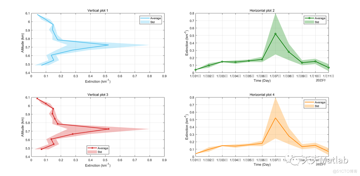
基于Matlab绘制带阴影区域的线附完整代码
⛄ 完整代码
clc
clear all
close all
X = [ 0.0397    0.0979    0.1479    0.1428    0.1596    0.1782  0.5229    0.2795    0.1346    0.1518    0.0685];
Y = [ 0    0.0296    0.0064    0.0230    0.0165    0.0356    0.2772   0.1100    0.0333    0.0355    0.0466];
Z = [6.0853    6.0254    5.9655    5.9057    5.8458    5.7859    5.7260    5.6662    5.6063    5.5464    5.4865];
Z2 = datetime(2023,1,1):datetime(2023,1,11);

figure;
nexttile;
ShadedPlot(X,Y,Z,'vertical'); % vertical plot
box on; grid on;
title('Vertical plot 1')
xlabel('Extinction (km^-^1)')
ylabel('Altitude (km)')

nexttile;
ShadedPlot(X,Y,Z2,'horizontal','Marker','o','Color','green'); % horizontal plot
box on; grid on;
xlabel('Time (Day)')
ylabel('Extinction (km^-^1)')
title('Horizontal plot 2')

nexttile;
ShadedPlot(X,Y,Z,'vertical','Marker','square','Color','red','Legend_Loc','south'); % vertical plot
box on; grid on;
title('Vertical plot 3')
xlabel('Extinction (km^-^1)')
ylabel('Altitude (km)')

nexttile;
ShadedPlot(X,Y,Z2,'horizontal','Marker','none','Color','orange'); % horizontal plot
box on; grid on;
xlabel('Time (Day)')
ylabel('Extinction (km^-^1)')
title('Horizontal plot 4')
function ShadedPlot( meanarray,disparray,array,orientation,varargin)%,orientation,name,color,marker )
%ShadedPlot - Plots the line with shaded region.
%
% Syntax:
% ShadedPlot(meanarray,disparray,array,varargin)
%
% Description:
% ShadedPlot() - Plots the line with shaded region under the line.
% Depending on the 'orientation', It is possible to have a vertical
% (e.g., altitude) or horizontal (e.g., time) representation.
%
% Inputs:
% meanarray - vector for the Line (Average Data)
% disparray - vector for the Shaded Region (Dispersion Data)
% array - vector for the y-axis (e.g., altitude) or the x-axis (e.g., datetime)
% orientation - orientation of the plot 'vertical' or 'horizontal'
% varargin - Custome parameters such as color,marker, markersize,
% displaynames, legend location
%
%
% Other m-files required: none
% Subfunctions: none
% MAT-files required: none
% Inspired from ploterr function, written by Brendan Hasz (haszx010@umn.edu) Apr 2018
% Author: Marion Ranaivombola
% email: marion.ranaivombola@univ-reunion.fr
% Date: 01-Sep-2021; Last revision: 10-Jan-2023
%
% Copyright (c) 2023, Marion Ranaivombola
% All rights reserved.
%% Colors
blue = [0.30 0.75 0.93];
red = [0.8300 0.1400 0.1400];
orange = [1.00 0.54 0.00];
purple = [0.7176 0.2745 1.0000];
green = [0.00,0.50,0.00];
black = [0 0 0];
gray = [0.5 0.5 0.5];
colors = [blue; red; orange; purple; green; black; gray];
%% Requiered parameters
p = inputParser;
p.KeepUnmatched = true;
addRequired(p, 'meanarray', @isnumeric);
addRequired(p, 'disparray', @isnumeric);
%% Defaults parameters
iscolor = @(x) (isvector(x) && length(x)==3) || ischar(x) || isscalar(x);
addParameter(p, 'Color', blue, iscolor);
addParameter(p, 'Marker', 'none', @ischar);
addParameter(p, 'MarkerSize',4, @isnumeric);
addParameter(p, 'EdgeAlpha',0,@isnumeric);
addParameter(p, 'FaceAlpha',0.3,@isnumeric);
addParameter(p, 'LineName', 'Average', @ischar);
addParameter(p, 'ShadedName', 'Std', @ischar);
addParameter(p, 'Legend_Loc','northeast',@ischar)
parse(p, meanarray, disparray, varargin{:});
Color = p.Results.Color;
Marker = p.Results.Marker;
MarkerSize = p.Results.MarkerSize;
EdgeAlpha = p.Results.EdgeAlpha;
FaceAlpha = p.Results.FaceAlpha;
LineName = p.Results.LineName;
ShadedName = p.Results.ShadedName;
Location = p.Results.Legend_Loc;
%Set Color
if ischar(Color)
try
eval(['Color=' Color ';']);
catch err
error([Color ' is not a valid color string'])
end
end
if isnumeric(Color) && isscalar(Color)
Color = colors(round(Color), :);
end
%% Set column vectors
% meanarray
result_meanarray = iscolumn(p.Results.meanarray);
if result_meanarray ==0
meanarray = p.Results.meanarray';
end
% disparray
result_disparray = iscolumn(p.Results.disparray);
if result_disparray ==0
disparray = p.Results.disparray';
end
% array
result_array = iscolumn(array);
if result_array ==0
array = array';
end
%% Set the Border of Shaded Region
posi = meanarray + disparray;
nega = meanarray - disparray;
%% Change NaN to Zero for Shaded Region
function OutArray = NaN2zero(matrix)
OutArray = matrix;
OutArray(isnan(OutArray))=0;
end
y1 = NaN2zero(nega);
y2 = NaN2zero(posi);
%% Plot shaded area
switch(orientation)
case('vertical')
hold on;
pa = patch([y1; flipud(y2)],[array ; flipud(array)],Color);
X = meanarray;
Y = array;
case('horizontal')
hold on;
pa = patch([array ; flipud(array)],[y1; flipud(y2)],Color);
X = array;
Y = meanarray;
end
pa.EdgeAlpha = EdgeAlpha;
pa.FaceAlpha = FaceAlpha;
pa.DisplayName = ShadedName;
switch(p.Results.Marker)
case('none')
po= plot(X,Y, ...
'DisplayName',LineName, ...
'LineWidth',2, ...
'Color',Color ,...
'LineStyle','-');
otherwise
po = plot(X,Y, ...
'DisplayName',LineName, ...
'LineWidth',2, ...
'Color',Color, ...
'MarkerFaceColor','w', ...
'MarkerSize',MarkerSize, ...
'LineStyle','-');
po.Marker = Marker;
end
hold off
legend([po pa],'Location',Location)
end⛄ 运行结果


 1530
1530


 被折叠的 条评论
为什么被折叠?
被折叠的 条评论
为什么被折叠?
 到【灌水乐园】发言


