系统辨识 Identification Algorithm（基础篇）

版权声明：本文为Fally J 幻灵原创文章，遵循 CC 4.0 BY-SA 版权协议，转载请附上原文出处链接和本声明。

原文链接：系统辨识 Identification Algorithm（基础篇）-CSDN博客

        由于原文公式不全，故转载于此并将公式代码转换过来，做了略微改动，但有些地方目前还看不懂，没有验证原文的正确性。为了避免错误排版，建议在电脑端阅读。

目录

基础知识

什么是系统辨识

辨识模型

噪声

矩阵运算

 模型

时间序列模型 Time series model

 方程误差模型 Equation error type model

输出误差模型 Output error type model

最小二乘法 Least Squares Principle

迭代最小二乘辨识 RLS identification

迭代最小二乘辨识的推导（对ARX模型）

最终结论 

几个重要概念

带遗忘因子的迭代最小二乘辨识算法 FF-RLS

数据饱和

带遗忘因子的RLS

基础篇总结

---

基础知识

什么是系统辨识

        根据测得的输入输出，通过最小化误差标准函数，确定数学模型中未知的参数取值

        Identification can be defined as the determination of a mathematical model from the observed input and output data by minimizing some error criterion function.

        四个基本要素：

• A data set 数据集
• A set of candidate models 模型类
• criterion function 指标函数
• optimizaiton approaches 优化方法

辨识模型

        在传递函数中，我们常用微分算子\(s\)的分式来表达输入输出之间的关系。在系统辨识中，我们根据移位算子\(z\)的差分方程来表达输入、输出、噪声之间的关系

\[ \begin{align}
&\text{forward shift operator} &zu(t)=u(t+1)\\
&\text{backward shift operator}&z^{-1}u(t)=u(t-1)
\end{align} \]

         在系统辨识算法中，为了让不同的情况，不同的算法有共通的体系结构，我们所有的算法均是基于辨识模型(identification model)进行推演

\[ y(t)=H_t\theta+v(t)\quad
\text{where }v(t) \text{ is white noise} \]

         辨识模型的特点：无参变量\已知量 = 带参变量*待辨识参数 + 白噪声

噪声

        随机变量：形容随机事件的数学描述

        随机过程：随时间变化的随机变量，依赖于时间\(t\)和事件\(\omega\)，当时间固定时，即随机变量

        白噪声 White Noise：

\[ \begin{align}
&\text{1) expectation is zero:}\quad E[v(t)]=0 \\
&\text{2) variance } E[v^2(t)] \text{ is time invarivant} \\
&\text{3) } E[v(t)-E[v(t)]](v(\tau)-E[v(\tau)])=0
\end{align} \]

         Question: which terms as follows belong to white noise if \( v(t) \) is white noise:

\[ \begin{align}
& \text{A}. zv(t) \\
& \text{B}. z^{-1}v(t) \\
& \text{C}. av(t) \\
& \text{D}. (a+bz^{-1})v(t)
\end{align} \]

        根据白噪声的定义和性质可知，ABC仍然属于白噪声，而D不满足第三个条件 

矩阵运算

•         \(f\)列向量对\(x\)列向量的偏导：

\[ \frac{\partial f}{\partial x} = \begin{bmatrix}
\dfrac{\partial f_1}{\partial x_1} & \dfrac{\partial f_2}{\partial x_1} & \cdots  & \dfrac{\partial f_m}{\partial x_1} \\
\dfrac{\partial f_1}{\partial x_2} & \dfrac{\partial f_2}{\partial x_2} & \cdots  & \dfrac{\partial f_m}{\partial x_2} \\
\vdots & \vdots & \ddots & \vdots \\
\dfrac{\partial f_1}{\partial x_n} & \dfrac{\partial f_2}{\partial x_n} & \cdots  & \dfrac{\partial f_m}{\partial x_n} \end{bmatrix} \]

•         \(f\)标量对\(x\)列向量的偏导：

\[ \frac{\partial f}{\partial x} =\begin{bmatrix}
\dfrac{\partial f}{\partial x_1} \\
\dfrac{\partial f}{\partial x_2} \\
\vdots \\
\dfrac{\partial f}{\partial x_n} \end{bmatrix} \] 

•         \(f\)列向量对\(x\)标量的偏导：

\[ \frac{\partial f}{\partial x}  = \begin{bmatrix}
\dfrac{\partial f_1}{\partial x} \\
\dfrac{\partial f_2}{\partial x} \\
\vdots \\
\dfrac{\partial f_m}{\partial x} \end{bmatrix} \]

•         Lemma 1

\[ \text{Given } A\in \mathbb{R}^{n \times n},\
f(x)=x^\top{}Ax,\text{ one has}\\
\frac{\partial f}{\partial x}=Ax+A^\top{}x \]

•         Lemma 2

 \[ \text{Given } A\in \mathbb{R}^{m \times n}, \
f(x) = Ax, \text{ one has} \\
\frac{\partial f}{\partial x} = A^\top{} \]

•         链式法则(chain rule)  

\[ \text{Let } x = \begin{bmatrix} x_1 \\ x_2 \\ \vdots \\ x_n \end{bmatrix},\
y = \begin{bmatrix} y_1 \\ y_2 \\ \vdots \\ x_r \end{bmatrix},\
z = \begin{bmatrix} z_1 \\ z_2 \\ \vdots \\ z_m \end{bmatrix},\
\text{where } z \text{ is a function of } y,\text{ which is in turn a function of }x. \text{ Then,}\\
 \frac{\partial z}{\partial x} = \frac{\partial y}{\partial x}\frac{\partial z}{\partial y} \]

---

 模型

(转载者注)本人对此章比较疑惑，建议结合其他文章阅读，如线性模型：AR、MA、ARMA、ARMAX、ARX、ARARMAX、OE、BJ等，【系统辨识】随机系统的数学模型

        系统辨识中的模型均采用差分方程 difference function 的形式表达，其中

\[ A(z)=1+\sum_{i=1}^{n_a} {a_i z^{-i}},\quad
B(z)=  \sum_{i=1}^{n_b} {b_i z^{-i}},\quad
C(z)=  \sum_{i=1}^{n_c} {c_i z^{-i}},\quad
D(z)=  \sum_{i=1}^{n_d} {d_i z^{-i}} \] 

        常用模型如下

时间序列模型 Time series model

• 自回归模型 AutoRegressive (AR) model

\[ \begin{align}
y(t)+a_{1}y(t-1)+a_{2}y(t-2)+\cdots+a_{n_{a}}y(t-n_{a})=v(t)\\
A(z)y(t)=v(t)
\end{align} \]

        其中\(v\)是白噪声，\(n_a\)是自回归信号的阶

• 滑动平均模型 Moving Average (MA) model

\[ \begin{align}
y(t)&=v(t)+d_{1}v(t-1)+d_{2}v(t-2)+...+d_{n_{d}}v(t-n_{d})\\
y(t)&=D(z)v(t)
\end{align} \]

• 自回归滑动平均模型 AutoRegressive Moving Average (ARMA) model

\[ \begin{align}
y(t)+a_{1}y(t-1)+a_{2}y(t-2)+...+a_{n_{a}}y(t-n_{a})
&=v(t)+d_{1}v(t-1)+d_{2}v(t-2)+...+d_{n_{d}}v(t-n_{d})\\
A(z)y(t)&=D(z)v(t)
\end{align} \]

• 确定性ARMA模型 Deterministic ARMA (DARMA) model 

\[ \begin{align}
y(t)+a_{1}y(t-1)+a_{2}y(t-2)+...+a_{n_{a}}y(t-n_{a})
&=u(t)+b_{1}u(t-1)+b_{2}u(t-2)+...+b_{n_{b}}u(t-n_{b})\\
A(z)y(t)&=B(z)u(t)
\end{align} \]

• 自回归整合滑动平均模型 AutoRegressive Integtated Moving Average (ARIMA) model

\[ A(z)(1-z^{-1})^{d}y(t)=D(z)v(t) \]

 方程误差模型 Equation error type model

        以下命名中的字母分别对应，输出信号类型、噪声类型、输入X

\[ \begin{align}
\text{General:}\quad &A(z)y(t)=B(z)u(t)+w(t)\\
\text{ARX:} \quad &A(z)y(t)=B(z)u(t)+v(t)\\
\text{ARMAX:} \quad &A(z)y(t)=B(z)u(t)+\frac{1}{C(z)}v(t)\\
\text{ARARMA(BJ):} \quad &A(z)y(t)=B(z)u(t)+\frac{D(z)}{C(z)}v(t)
\end{align} \]

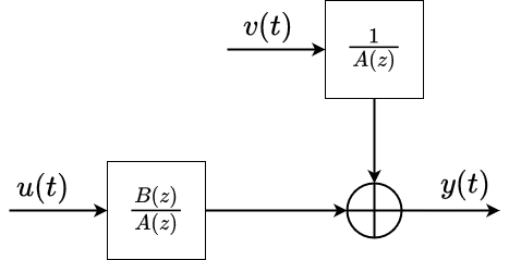
输出误差模型 Output error type model

         以下命名中的字母分别对应，输出OE、输入类型、噪声类型

\[ \begin{align}
\text{General:}\quad &y(t)=\frac{B(z)}{A(z)}u(t)+w(t)\\
\text{OE:} \quad &y(t)=\frac{B(z)}{A(z)}u(t)+v(t)\\
\text{OEMA:} \quad &y(t)=\frac{B(z)}{A(z)}u(t)+D(z)v(t)\\
\text{OEARMA(BJ):} \quad &y(t)=\frac{B(z)}{A(z)}u(t)+\frac{D(z)}{C(z)}v(t)\\
\end{align} \]

---

最小二乘法 Least Squares Principle

        此章为最小二乘法的推导过程，作为系统辨识算法推理的基础，详见最小二乘估计 （转载者注：然而这篇文章的公式也不能正常显示，于是本人也做了转载，可见最小二乘算法）

---

迭代最小二乘辨识 RLS identification

        最小二乘辨识算法的核心，在于将现有模型转化为辨识模型(identification model)用以参数辨识

\[ y(t)=H_t\theta+v(t)\quad
\text{where }v(t) \text{ is white noise} \] 

迭代最小二乘辨识的推导（对ARX模型）

\[ A(z)y(t)=B(z)u(t)+v(t) \\
A(z)=1+\sum_{i=1}^{n_a}{a_iz^{-i}};\quad B(z)=1+\sum_{i=1}^{n_b}{b_i}z^{-i} \]

\[ \text{We define}\quad \theta =
\begin{bmatrix}
a_1 & a_2 & \cdots & a_{n_a} & b_1 & b_2 & \cdots & b_{n_b}
\end{bmatrix}^{\top} \]

\[ \varphi(t)=\begin{bmatrix} -y(t-1) & -y(t-2) & \cdots & -y(t-n_a) & u(t-1) & u(t-2) & \cdots & u(t-n_b) \end{bmatrix}^{\top}  \]

ARX模型

        为了凑成辨识模型，我们定义\( \theta \)和\( \varphi \)以便后期计算，可得相应的辨识模型

\[ \begin{align}
Y_t = \begin{bmatrix} y(1) \\ y(2) \\ \vdots \\y(t)\end{bmatrix} \in \mathbb{R}^t,\
H_t &= \begin{bmatrix} \varphi^\top{}(1) \\ \varphi^\top{}(2)\\ \vdots \\ \varphi^\top{}(t)\end{bmatrix} \in \mathbb{R}^{t \times n},\
V_t = \begin{bmatrix} v(1) \\ v(2) \\ \vdots \\v(t) \end{bmatrix} \in \mathbb{R}^t,\\
\text{identification model:}\quad
Y_t &= H_t\theta+V_t\\
\text{quadratic criterion function:}\quad
J(\theta) &= V_t^\top{} V_t\\
&=(Y_t-H_t\theta)^\top{}(Y_t-H_t\theta)
\end{align}  \]

        根据最小二乘法中得到的结论，参数\( \theta \)的最小二乘估计为

\[ \hat{\theta}(t)=\hat{\theta}_{LS}(t)=(H_t^\top{}H_t)^{-1}H_t^\top{}Y_t \]

        据此，将LSE中求逆的部分单独定义为

\[ P(t) = (H_t^{\top{}} H_t)^{-1} \]

        为了保证算法的递推性，需要将LSE中的各变量递推关系式写出，如下

\[ \begin{align}
P^{-1}(t) &= H_t^\top{}H_t = \sum_{i=1}^{t}{\varphi(i)\varphi^\top(i)} = P^{-1}(t-1)+\varphi(t)\varphi^\top(t) \tag{1.1}\\
Y_t &= \begin{bmatrix} y(1) \\ y(2) \\ \vdots \\ y(t-1) \\ y(t) \end{bmatrix}
=\begin{bmatrix} Y_{t-1} \\ y(t) \end{bmatrix} \in \mathbb{R}^t;\\
H_t &= \begin{bmatrix} \varphi^\top(1) \\ \varphi^\top(2) \\ \vdots \\ \varphi^\top(t-1) \\ \varphi^\top(t) \end{bmatrix}
=\begin{bmatrix} H_{t-1} \\ \varphi^\top(t) \end{bmatrix} \in \mathbb{R}^{t \times n}
\end{align} \]

        上述公式表示了各个变量在当前时刻与前一个时刻的递推关系，我们将上述递推关系代入LSE中得到递推的LSE（此步骤目的是得到 \( \theta(t) \)与\( \theta(t-1) \)之间的递推关系）

 \[ \begin{align}
\hat{\theta}(t)&=(H_t^\top{}H_t)^{-1}H_t^\top{}Y_t\\
&=P(t) \begin{bmatrix} H_{t-1} \\ \varphi^\top{}(t) \end{bmatrix}^\top{}
\begin{bmatrix} Y_{t-1} \\ y(t) \end{bmatrix}\\
&=P(t)( H_{t-1}^\top{} Y_{t-1} + \varphi(t)y(t))
\end{align} \]

\[ \begin{align}
\because \
I_t &= P(t)P^{-1}(t-1) + P(t)\varphi^\top{}(t)\varphi(t)\\
\therefore\
\hat{\theta}(t) &= P(t)(P^{-1}(t-1)P(t-1)H_{t-1}^\top{}Y_{t-1} + \varphi(t)y(t))\\
&=(I_t-P(t)\varphi^\top{}(t)\varphi(t))(P(t-1)H_{t-1}^\top{}Y_{t-1})+P(t)\varphi(t)y(t)\\
&=(I_t-P(t)\varphi^\top{}(t)\varphi(t))\hat{\theta}(t-1)+P(t)\varphi(t)y(t)\\
&=\hat{\theta}(t-1)+P(t)\varphi(t)[y(t)-\varphi^\top{}(t)\hat{\theta}(t-1)]
\end{align} \]

        经过上面复杂的推导，终于获得了递推最小二乘估计(Recursive Least Squares Estimation)算法

最终结论 

        由于矩阵求逆在实际运算中非常不友好，甚至不能保证可逆，因此引入以下矩阵多项式求逆算法：

\[ (A+BC)^{-1}=A^{-1}-A^{-1}B(I+CA^{-1}B)^{-1}CA^{-1} \]

        代入到\( P(t) \)的递推关系式中，如下

 \[ \begin{align}
P^{-1}(t)&=P^{-1}(t-1)+\varphi(t)\varphi^\top{}(t)\\
\Rightarrow P(t)&=P(t-1)-\frac{P(t-1)\varphi(t)\varphi^\top(t)P(t-1)}{1+\varphi^\top{}(t)P(t-1)\varphi(t)}
\end{align} \]

        \( P(t) \)称为协方差矩阵(covariance matrix)

        为了表示方便，下面定义一个新的变量\( L(t) \)

\[ \begin{align}
L(t)&=P(t)\varphi(t)\\
&=\frac{P(t-1)\varphi(t)}{1+\varphi^\top{}(t)P(t-1)\varphi(t)}
\end{align} \]

        于是，可以得到递推最小二乘辨识的完整算法：

\[ \begin{align}
\text{Algorithm CAR-RLS:}\\
\hat{\theta}(t)&=\hat{\theta}(t-1)+P(t)\varphi(t)[y(t)-\varphi^\top{}(t)\hat{\theta}(t-1)]\\
L(t)&=\frac{P(t-1)\varphi(t)}{1+\varphi^\top{}T(t)P(t-1)\varphi(t)}\\
P(t)&=[I-L(t)\varphi^\top{}(t)]P(t-1);\ P(0)=p_0I\\
\varphi(t)&=\begin{bmatrix}-y(t-1) & -y(t-2) & \cdots & -y(t-n_a)& u(t-1)& u(t-2)& ...& u(t-n_b)\end{bmatrix} ^\top{} \tag{1.2}
\end{align} \]

几个重要概念

        针对 RLSE 中各部分物理含义如下图所示

        其中，根据\( P(t) \)的递推公式1.1，有下述情况需要考虑

 \[ \begin{align}
P(t)&=[\frac{1}{p_0}I+\sum_{i=1}^{t}{\varphi(i)\varphi^\top{}(i)}]^{-1}\\
&=[\frac{1}{p_0}I+H_t^\top{} H_t]^{-1}\\
\xrightarrow[]{\text{let }p_0\rightarrow \infty }&\approx (H_t^\top{} H_t)^{-1}=P(t)
\end{align} \]

        可见，当且仅当\( p_0 \)取较大值时，\( P(t) \)才能符合原有定义，否则算法会与实际值产生较大偏差

        除此之外，在此区分定义两个概念： 

        新息(innovation)：\( e(t) = y(t) - \varphi^\top{}(t) \hat{\theta}(t-1) \)

        残差(residual)： \( \hat{\varepsilon}(t) = y(t) - \varphi^\top{}(t) \hat{\theta}(t) \)

        残差与新息的关系： 

 \[ \begin{align}
\varepsilon(t)&=y(t)-\varphi^\top{}(t)[\hat{\theta}(t-1)+L(t)e(t)]\\
&=[1-\frac{\varphi^\top{}(t)P(t)\varphi(t)}{1+\varphi^\top{}(t)P(t)\varphi(t)}]e(t)<e(t)\\
&=\frac{1}{1+\varphi^\top{}(t)P(t)\varphi(t)}e(t)>0\\
\therefore 0&<\frac{\varepsilon(t)}{e(t)}<1
\end{align} \]

带遗忘因子的迭代最小二乘辨识算法 FF-RLS

数据饱和

        根据RLS算法，我们可以有以下推导

\[ \begin{align}
&\because P(t)-P(t-1)=-\frac{P(t-1)\varphi(t)\varphi^\top(t)P(t-1)}{1+\varphi^\top(t)P(t-1)\varphi(t)}<0\\
&\therefore P(t) \text{ is monotonous decreasing}\\
\text{and }&\because \text{covariance  matrix } P(t)=(H_t^\top H_t)^{-1}>0\\
&\therefore \lim_{t \rightarrow \infty}P(t)=0\\
\text{then }&\hat{\theta}(t)=\hat{\theta}(t-1)+P(t-1)\varphi(t)e(t)\xrightarrow[]{t\rightarrow\infty}\hat{\theta}(t-1)
\end{align} \]

        从上述推理可以发现，由于协方差矩阵\( P \)具有正定且单调递减的特性，会随着时间的增长最终趋于零，从而导致后面新加入的数据，对RLSE的影响越来越小

        这种情况下，对于一个数据集，如果有效数据集中在前面，不会对算法结果产生影响，正常运行；然而，如果有效数据集中在后面，则RLS会根据前面的无效数据获得结果，且后面的有效数据因为算法这一问题，无法修正结果，此时RLS的最终结果就是错误的。针对这种，新加入数据无法正常修正辨识结果的现象，称为数据饱和(data saturation)

         data saturation: a phenomenon in which the new data have no attribution to improve the estimation of the parameter \( \theta \)

带遗忘因子的RLS

        为了解决数据饱和的问题，针对迭代算法，我们在每一次运算时，可以通过手动削弱之前估计值的影响，来保证新加入的数据可以修正结果

\[ y_t = \begin{bmatrix} \rho Y_{t-1} \\ y(t) \end{bmatrix} \in \mathbb{R}^t,\
H_t = \begin{bmatrix} \rho H_{t-1} \\ \varphi^\top(t) \end{bmatrix} \]

        其中，\( 0<\rho<1 \)加权给过去的数据，用以削弱之前数据的影响，则之前的RLS算法(1.2)均发生改变

\[ \begin{align}
P^{-1}(t)
&=\begin{bmatrix} \rho H_{t-1} \\ \varphi^\top{}(t) \end{bmatrix}^\top
\begin{bmatrix} \rho H_{t-1} \\ \varphi^\top{}(t) \end{bmatrix}\\
&=\rho^2H_{t-1}^\top{}H_{t-1}+\varphi(t)\varphi^\top(t)\\
&=\rho^2P^{-1}(t-1)+\varphi(t)\varphi^\top(t)\\
\Leftrightarrow P(t)
&=\frac{1}{\rho^2}[I-\frac{P(t-1)\varphi(t)\varphi^\top(t)}{\rho^2+\varphi^\top(t)P(t-1)\varphi(t)}]P(t-1)\\
\xrightarrow[]{ \text{denote } \rho^2=\lambda}
&=\frac{1}{\lambda}[I-L(t)\varphi^\top(t)]P(t-1)\\
\text{where }L(t)
&=\frac{P(t-1)\varphi(t)}{\lambda+\varphi^\top(t)P(t-1)\varphi(t)}
\end{align} \]

        根据上面求得的参数，RLSE为

\[ \begin{align}
\hat{\theta}(t)
&= P(t) \begin{bmatrix} \rho H_{t-1} \\ \varphi^\top{}(t) \end{bmatrix}^\top
\begin{bmatrix} \rho Y_{t-1} \\ y(t) \end{bmatrix}\\
&= P(t)(\rho^2 H_{t-1}^\top{}Y_{t-1}+\varphi(t)y(t))\\
&= \hat{\theta}(t-1)+P(t-1)\varphi(t)[y(t)-\varphi^\top(t)\hat{\theta}(t-1)]
\end{align} \]

        可以发现，参数\( P \)和\( L \)均发生了改变，而RLSE的形式却没有变化

        不难发现，当引入了 遗忘因子 \( \lambda \) 后，\( P \)的正定性不改变，但是却不在满足单调递减的性质，也就不在趋于零了。数据饱和得以解决

        上图可以发现，采用传统的RLS算法，最后参数几乎不再变化，即几乎不受新数据影响；而遗忘因子较小时，参数误差呈发散状，达不到理想结果。一般而言，\( \lambda = 0.98 \)效果较优，既可以削弱旧数据影响，还可以避免过快的衰减

        这种通过加入遗忘因子，来增加新数据权重，削弱旧数据影响的方式，称为带有遗忘因子的递推最小二乘辨识算法FF-RLS(Forgetting factor recursive least squares identification algorithm)

        FF-RLS: the idea that introduce a factor for old data, in order to increase the contribution of new data and to reduce the influence of old data

---

基础篇总结

        以上主要是针对系统辨识的目的、原理、基本推导方法进行总结归纳。

        主要掌握通用RLS算法(1.2)，以及数据饱和现象及其应对方式，知晓遗忘因子的作用和对RLS算法的影响