全球0.05°日光诱导叶绿素荧光数据（2000-2022）处理

国家青藏高原科学数据中心

数据来源↑  感谢张尧老师团队生产的CSIF！

1、均值合成到8d

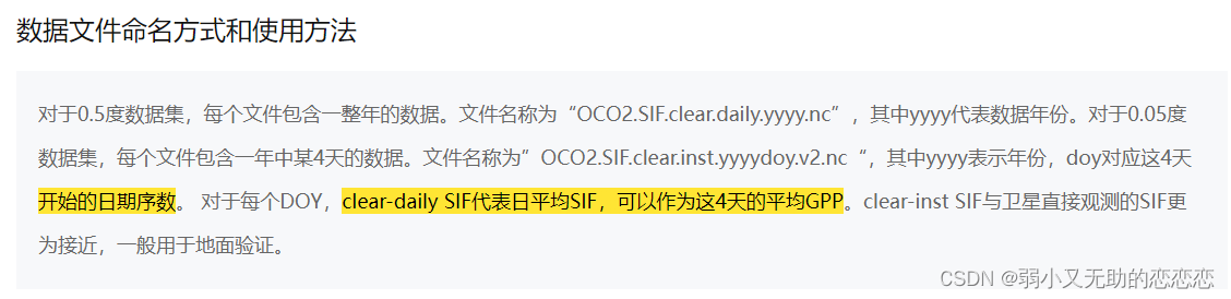
原始数据为每4天的nc文件，我选择了 clear-daily SIF，好像看到过这个的质量高于clear-inst SIF。

我想要合成到8天的，于是用python进行了均值合成：

import xarray as xr

# 打开4个NetCDF文件
ds1 = xr.open_dataset('D:/Data_Drought_LL/CSIF/python_0122/2016/SIF.clear.inst.2016249.nc')
ds2 = xr.open_dataset('D:/Data_Drought_LL/CSIF/python_0122/2017/SIF.clear.inst.2017249.nc')

# 计算平均值
average_ds = xr.concat([ds1, ds2, ds3, ds4], dim='time').mean(dim='time')

# 关闭打开的文件
ds1.close()
ds2.close()

# 将结果保存到新的NetCDF文件
average_ds.to_netcdf('D:/Data_Drought_LL/CSIF/python_0122/Multimean/SIF_multi249.nc')

2、计算对应doy的多年平均值（我自己的研究需要）

同样采用均值合成

import xarray as xr

# 打开4个NetCDF文件
ds1 = xr.open_dataset('D:/Data_Drought_LL/CSIF/python_0122/2016/SIF.clear.inst.2016249.nc')
ds2 = xr.open_dataset('D:/Data_Drought_LL/CSIF/python_0122/2017/SIF.clear.inst.2017249.nc')
ds3 = xr.open_dataset('D:/Data_Drought_LL/CSIF/python_0122/2018/SIF.clear.inst.2018249.nc')
ds4 = xr.open_dataset('D:/Data_Drought_LL/CSIF/python_0122/2021/SIF.clear.inst.2021249.nc')

# 计算平均值
average_ds = xr.concat([ds1, ds2, ds3, ds4], dim='time').mean(dim='time')

# 关闭打开的文件
ds1.close()
ds2.close()

# 将结果保存到新的NetCDF文件
average_ds.to_netcdf('D:/Data_Drought_LL/CSIF/python_0122/Multimean/SIF_multi249.nc')

以上两种都是只能自己手动修改doy的笨方法，因为不会写python循环==

3、NC文件转tif

我还是觉得arcgis 模型构建器更方便，参考下面的博文转了tif文件。

在ArcGIS中使用建模批量将nc文件转换为tif格式并进行裁剪_gis批量拆分nc-CSDN博客

           同样不会改代码，师姐的python代码如下，供参考：

# -*- encoding: utf-8 -*-
'''
@File    :   nc2tif.py
@Time    :   2023/09/19 09:51:10
@Author  :   HMX
@Version :   1.0
@Contact :   kzdhb8023@163.com
'''

# here put the import lib
from osgeo import gdal, osr
import xarray as xr
import pandas as pd
import numpy as np
import os
import warnings

warnings.filterwarnings("ignore")

def nc2tif(fn,outfp):
    '''nc转tif

    :param fn: nc文件路径
    :param outfp: 转换后tif文件夹
    '''
    ds = xr.open_dataset(fn)
    # print(ds)
    df = pd.DataFrame({'lon':ds.longitude, 'lat':ds.latitude,'xch4':ds.xch4})
    print(df.lon.min(),df.lat.max())
    # print(df)

    # 定义栅格的分辨率
    resolution = 0.0628

    # 构建网格
    lonbin = np.arange(df.lon.min()-resolution/2,180.1,resolution)
    latbin = np.arange(df.lat.min()-resolution/2,90.1,resolution)
    df['lonbin'] = pd.cut(df['lon'], bins = lonbin, right = False)
    df['latbin'] = pd.cut(df['lat'], bins = latbin, right = False)
    df['x'] = [interval.left for interval in df['lonbin']]
    df['y'] = [interval.left for interval in df['latbin']]
    res = df.groupby(['x', 'y'])['xch4'].mean().reset_index()
    res.reset_index(inplace=True)
    # print(res)

    # 计算栅格的范围
    lon_min, lat_min, lon_max, lat_max = res['x'].min(), res['y'].min(), res['x'].max(), res['y'].max()
    # print(lon_min, lat_min, lon_max, lat_max)
    width = int((lon_max - lon_min) / 0.0628) + 1
    height = int((lat_max - lat_min) / 0.0628) + 1

    # 创建一个新的栅格数据集
    outfn = os.path.join(outfp,os.path.basename(fn).replace('.nc','.tif'))
    driver = gdal.GetDriverByName('GTiff')
    dataset = driver.Create(outfn, width, height, 1, gdal.GDT_Float32)

    # 设置地理转换
    dataset.SetGeoTransform((lon_min, resolution, 0, lat_max, 0, -resolution))

    # 设置坐标系
    srs = osr.SpatialReference()
    srs.ImportFromEPSG(4326)  # WGS84
    dataset.SetProjection(srs.ExportToWkt())

    # 获取栅格的第一个波段
    band = dataset.GetRasterBand(1)

    # 创建一个空的栅格数据
    raster = np.zeros((height, width), dtype=np.float32)
    # print(raster.shape)
    # 将dataframe的数据填充到栅格中
    # 将 data frame 的数据填充到栅格中
    for i in range(len(res)):
        col = int((res['x'][i] - lon_min + resolution / 2) / resolution)
        row = int((lat_max - res['y'][i] + resolution / 2) / resolution)
        row = min(row, height - 1)  # 添加的代码
        col = min(col, width - 1)  # 添加的代码
        raster[row, col] = res['xch4'][i]
    # 将栅格数据写入到波段中
    band.WriteArray(raster)
    band.SetNoDataValue(0.)
    # 保存并关闭数据集
    dataset = None


if __name__ == '__main__':
    # 待处理nc文件夹路径
    infp = r'G:\Bremen_tropomi\L2-CH4-CO-TROPOMI-WFMD-202103' \
           r''
    # 输出tif文件夹路径
    outfp = r'G:\TD\Bremen_tropomi\2021_perday_0.0628'
    for f in os.listdir(infp):
        if f.endswith('.nc'):
            fn = os.path.join(infp, f)
            nc2tif(fn,outfp)
    print('ok')

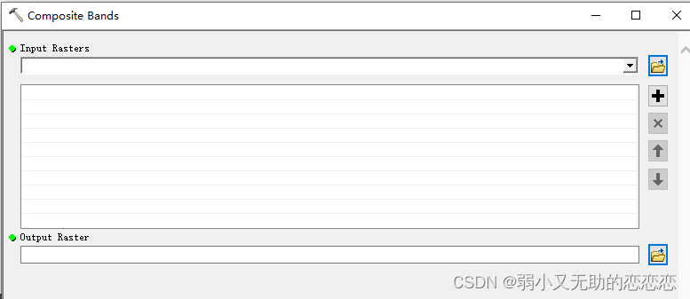
4、单波段多个image（tiff数据）合成为多波段的一个栅格数据

（这步主要是因为我后续需要上传到GEE计算时间序列，而多个数据上传很慢。）

用到了arcgis的波段合成工具：特别需要注意，这个批量拉很多数据进来是乱序的！！！需要自己手动调整排列好波段！！

5、GEE上将多波段image变成单波段的Imagecollection

GEE上，如何把arcgis中处理好的多波段数据变成单波段的一个Imagecollection，image中的每个band为一张image？

同时，原始数据中没有时间属性，我希望在Imagecollection中给每张 image 增加时间属性，然后统一波段名称：

// 获取波段名列表
var bandNames = image.bandNames();          // image是自己上传的多波段数据

// 获取影像的日期
var startDate = ee.Date('2022-01-01');      // 设定第一张image的时间，其他波段为每8天一张
var interval = 8; // 每8天获取一个影像

// 创建一个函数，将每个波段转换为单波段影像并设置日期信息
var convertToSingleBandWithDate = function(bandName) {
  // 计算当前波段的日期
  var date = startDate.advance(ee.Number(bandNames.indexOf(bandName)).multiply(interval), 'day');
  
  // 选择当前波段
  var singleBandImage = image.select([bandName]);
  
  // 设置单波段影像的属性，包括日期信息
  singleBandImage = singleBandImage.set({
    'system:index': date.format('YYYYMMDD'),
    'system:time_start': date.millis(),
    'date': date
  });
    // 将波段重命名为"b1"
  singleBandImage = singleBandImage.rename('b1');   // 这步如果注释掉，波段名称是各不相同的
  return singleBandImage;
};

// 使用map函数将所有波段转换为单波段影像
var singleBandCollection = ee.ImageCollection(bandNames.map(convertToSingleBandWithDate))
                          .map(function(img){
                            return img.clip(table)    // table为研究区矢量
                          });
print(singleBandCollection);

print('MultiMean',ui.Chart.image.series(singleBandCollection, table, ee.Reducer.mean(), 5550));