深度学习高级，Keras多输入和混合数据实现回归模型，2024年最新腾讯社招面试题目

先自我介绍一下，小编浙江大学毕业，去过华为、字节跳动等大厂，目前阿里P7

深知大多数程序员，想要提升技能，往往是自己摸索成长，但自己不成体系的自学效果低效又漫长，而且极易碰到天花板技术停滞不前！

因此收集整理了一份《2024年最新Python全套学习资料》，初衷也很简单，就是希望能够帮助到想自学提升又不知道该从何学起的朋友。

既有适合小白学习的零基础资料，也有适合3年以上经验的小伙伴深入学习提升的进阶课程，涵盖了95%以上Python知识点，真正体系化！

由于文件比较多，这里只是将部分目录截图出来，全套包含大厂面经、学习笔记、源码讲义、实战项目、大纲路线、讲解视频，并且后续会持续更新

如果你需要这些资料，可以添加V获取：vip1024c （备注Python）

正文

continuous = [“bedrooms”, “bathrooms”, “area”]

performin min-max scaling each continuous feature column to

the range [0, 1]

cs = MinMaxScaler()

trainContinuous = cs.fit_transform(train[continuous])

testContinuous = cs.transform(test[continuous])

one-hot encode the zip code categorical data (by definition of

one-hot encoding, all output features are now in the range [0, 1])

zipBinarizer = LabelBinarizer().fit(df[“zipcode”])

trainCategorical = zipBinarizer.transform(train[“zipcode”])

testCategorical = zipBinarizer.transform(test[“zipcode”])

construct our training and testing data points by concatenating

the categorical features with the continuous features

trainX = np.hstack([trainCategorical, trainContinuous])

testX = np.hstack([testCategorical, testContinuous])

return the concatenated training and testing data

return (trainX, testX)

此函数通过 sklearn-learn 的 MinMaxScaler将最小-最大缩放应用于连续特征。

然后，计算分类特征的单热编码，这次是通过 sklearn-learn 的 LabelBinarizer。 然后连接并返回连续和分类特征。

加载图像数据集

==================================================================

图 6：我们模型的一个分支接受单个图像 - 来自家中的四张图像的蒙太奇。 使用蒙太奇与输入到另一个分支的数字/类别数据相结合，我们的模型然后使用回归来预测具有 Keras 框架的房屋的价值。

下一步是定义一个辅助函数来加载我们的输入图像。 再次打开 datasets.py 文件并插入以下代码：

def load_house_images(df, inputPath):

initialize our images array (i.e., the house images themselves)

images = []

loop over the indexes of the houses

for i in df.index.values:

find the four images for the house and sort the file paths,

ensuring the four are always in the same order

basePath = os.path.sep.join([inputPath, “{}_*”.format(i + 1)])

housePaths = sorted(list(glob.glob(basePath)))

initialize our list of input images along with the output image

after combining the four input images

inputImages = []

outputImage = np.zeros((64, 64, 3), dtype=“uint8”)

loop over the input house paths

for housePath in housePaths:

load the input image, resize it to be 32 32, and then

update the list of input images

image = cv2.imread(housePath)

image = cv2.resize(image, (32, 32))

inputImages.append(image)

tile the four input images in the output image such the first

image goes in the top-right corner, the second image in the

top-left corner, the third image in the bottom-right corner,

and the final image in the bottom-left corner

outputImage[0:32, 0:32] = inputImages[0]

outputImage[0:32, 32:64] = inputImages[1]

outputImage[32:64, 32:64] = inputImages[2]

outputImage[32:64, 0:32] = inputImages[3]

add the tiled image to our set of images the network will be

trained on

images.append(outputImage)

return our set of images

return np.array(images)

load_house_images 函数有三个目标：

• 加载房价数据集中的所有照片。 回想一下，我们每个房子都有四张照片（图 6）。

• 从四张照片生成单个蒙太奇图像。 蒙太奇将始终按照您在图中看到的方式排列。

• 将所有这些家庭蒙太奇附加到列表/数组并返回到调用函数。

我们定义了接受 Pandas 数据框和数据集 inputPath 的函数。

初始化图像列表。 我们将使用我们构建的所有蒙太奇图像填充此列表。 在我们的数据框中循环房屋。 在循环内部， 获取当前房屋的四张照片的路径。

执行初始化。 我们的 inputImages 将以列表形式包含每条记录的四张照片。 我们的 outputImage 将是照片的蒙太奇（如图 6 所示）。 循环 4 张照片： 加载、调整大小并将每张照片附加到 inputImages。 使用以下命令为四个房屋图像、创建平铺（蒙太奇）： 左上角的浴室图片。 右上角的卧室图片。 右下角的正面视图。 左下角的厨房。 将平铺/蒙太奇 outputImage 附加到图像。 跳出循环，我们以 NumPy 数组的形式返回所有图像。

定义模型

===============================================================

使用 Keras 的功能 API 构建的多输入和混合数据网络。

为了构建多输入网络，我们需要两个分支： 第一个分支将是一个简单的多层感知器 (MLP)，旨在处理分类/数字输入。 第二个分支将是一个卷积神经网络，用于对图像数据进行操作。 然后将这些分支连接在一起以形成最终的多输入 Keras 模型。 我们将在下一节中构建最终的串联多输入模型——我们当前的任务是定义两个分支。

打开models.py文件并插入以下代码：

import the necessary packages

from tensorflow.keras.models import Sequential

from tensorflow.keras.layers import BatchNormalization

from tensorflow.keras.layers import Conv2D

from tensorflow.keras.layers import MaxPooling2D

from tensorflow.keras.layers import Activation

from tensorflow.keras.layers import Dropout

from tensorflow.keras.layers import Dense

from tensorflow.keras.layers import Flatten

from tensorflow.keras.layers import Input

from tensorflow.keras.models import Model

def create_mlp(dim, regress=False):

define our MLP network

model = Sequential()

model.add(Dense(8, input_dim=dim, activation=“relu”))

model.add(Dense(4, activation=“relu”))

check to see if the regression node should be added

if regress:

model.add(Dense(1, activation=“linear”))

return our model

return model

导入。您将在此脚本中看到每个导入的函数/类。

分类/数值数据将由一个简单的多层感知器 (MLP) 处理。 MLP在create_mlp 定义。 在本系列的第一篇文章中详细讨论过，MLP 依赖于 Keras Sequential API。我们的 MLP 非常简单，具有：

• 具有 ReLU 激活功能的全连接（密集）输入层。

• 一个完全连接的隐藏层，也有 ReLU 激活。

• 最后，带有线性激活的可选回归输出。

虽然我们在第一篇文章中使用了 MLP 的回归输出，但它不会在这个多输入、混合数据网络中使用。您很快就会看到，我们将明确设置 regress=False，即使它也是默认值。回归实际上稍后会在整个多输入、混合数据网络的头部执行（图 7 的底部）。 现在让我们定义网络的右上角分支，一个 CNN：

def create_cnn(width, height, depth, filters=(16, 32, 64), regress=False):

initialize the input shape and channel dimension, assuming

TensorFlow/channels-last ordering

inputShape = (height, width, depth)

chanDim = -1

define the model input

inputs = Input(shape=inputShape)

loop over the number of filters

for (i, f) in enumerate(filters):

if this is the first CONV layer then set the input

appropriately

if i == 0:

x = inputs

CONV => RELU => BN => POOL

x = Conv2D(f, (3, 3), padding=“same”)(x)

x = Activation(“relu”)(x)

x = BatchNormalization(axis=chanDim)(x)

x = MaxPooling2D(pool_size=(2, 2))(x)

create_cnn 函数处理图像数据并接受五个参数：

• width ：输入图像的宽度（以像素为单位）。

• height ：输入图像有多少像素高。

• depth ：输入图像中的通道数。 对于RGB彩色图像，它是三个。

• 过滤器：逐渐变大的过滤器的元组，以便我们的网络可以学习更多可区分的特征。

• regress ：一个布尔值，指示是否将完全连接的线性激活层附加到 CNN 以用于回归目的。

模型的输入是通过 inputShape 定义的。 从那里我们开始循环过滤器并创建一组 CONV => RELU > BN => POOL 层。 循环的每次迭代都会附加这些层。 如果您不熟悉，请务必查看使用 Python 进行计算机视觉深度学习入门包中的第 11 章，以获取有关这些层类型的更多信息。

让我们完成构建我们网络的 CNN 分支：

flatten the volume, then FC => RELU => BN => DROPOUT

x = Flatten()(x)

x = Dense(16)(x)

x = Activation(“relu”)(x)

x = BatchNormalization(axis=chanDim)(x)

x = Dropout(0.5)(x)

apply another FC layer, this one to match the number of nodes

coming out of the MLP

x = Dense(4)(x)

x = Activation(“relu”)(x)

check to see if the regression node should be added

if regress:

x = Dense(1, activation=“linear”)(x)

construct the CNN

model = Model(inputs, x)

return the CNN

return model

我们展平下一层，然后添加一个带有 BatchNormalization 和 Dropout 的全连接层。

应用另一个全连接层来匹配来自多层感知器的四个节点。 匹配节点的数量不是必需的，但它确实有助于平衡分支。

检查是否应附加回归节点； 然后相应地添加它。 同样，我们也不会在这个分支的末尾进行回归。 回归将在多输入、混合数据网络的头部执行（图 7 的最底部）。

最后，模型是根据我们的输入和我们组装在一起的所有层构建的x

。 然后我们可以将 CNN 分支返回给调用函数。 现在我们已经定义了多输入 Keras 模型的两个分支，让我们学习如何组合它们！

使用 Keras 进行多输入

=========================================================================

我们现在准备构建能够处理多个输入和混合数据的最终 Keras 模型。 这是分支合并的地方，也是“魔法”最终发生的地方。训练也将在此脚本中进行。 创建一个名为 mix_training.py 的新文件，打开它，并插入以下代码：

import the necessary packages

from pyimagesearch import datasets

from pyimagesearch import models

from sklearn.model_selection import train_test_split

from tensorflow.keras.layers import Dense

from tensorflow.keras.models import Model

from tensorflow.keras.optimizers import Adam

from tensorflow.keras.layers import concatenate

import numpy as np

import argparse

import locale

import os

construct the argument parser and parse the arguments

ap = argparse.ArgumentParser()

ap.add_argument(“-d”, “–dataset”, type=str, required=True,

help=“path to input dataset of house images”)

args = vars(ap.parse_args())

首先处理我们的导入和命令行参数。 值得注意的进口包括：

• 数据集：我们三个方便的函数，用于加载/处理 CSV 数据和加载/预处理房屋数据集中的房屋照片。

• 模型：我们的 MLP 和 CNN 输入分支，它们将用作我们的多输入混合数据。

• train_test_split ：一个 scikit-learn 函数，用于构建我们的训练/测试数据拆分。

• concatenate ：一个特殊的 Keras 函数，它将接受多个输入。

• argparse ：处理解析命令行参数。

加载数值/分类数据和图像数据：

construct the path to the input .txt file that contains information

on each house in the dataset and then load the dataset

print(“[INFO] loading house attributes…”)

inputPath = os.path.sep.join([args[“dataset”], “HousesInfo.txt”])

df = datasets.load_house_attributes(inputPath)

load the house images and then scale the pixel intensities to the

range [0, 1]

print(“[INFO] loading house images…”)

images = datasets.load_house_images(df, args[“dataset”])

images = images / 255.0

在这里，我们将 House Prices 数据集加载为 Pandas 数据。

然后我们加载了我们的图像并将它们缩放到范围 [0, 1]。

partition the data into training and testing splits using 75% of

the data for training and the remaining 25% for testing

print(“[INFO] processing data…”)

split = train_test_split(df, images, test_size=0.25, random_state=42)

(trainAttrX, testAttrX, trainImagesX, testImagesX) = split

find the largest house price in the training set and use it to

scale our house prices to the range [0, 1] (will lead to better

training and convergence)

maxPrice = trainAttrX[“price”].max()

trainY = trainAttrX[“price”] / maxPrice

testY = testAttrX[“price”] / maxPrice

process the house attributes data by performing min-max scaling

on continuous features, one-hot encoding on categorical features,

and then finally concatenating them together

(trainAttrX, testAttrX) = datasets.process_house_attributes(df,

trainAttrX, testAttrX)

4:1的比例切分训练集和测试集。 从训练集中找到 maxPrice 并相应地缩放训练和测试数据。 将定价数据设置在 [0, 1] 范围内会导致更好的训练和收敛。

最后，我们继续通过对连续特征执行最小-最大缩放和对分类特征执行单热编码来处理我们的房屋属性。 process_house_attributes 函数处理这些操作并将连续特征和分类特征连接在一起，返回结果。

连接网络分支完成多输入 Keras 网络模型：

create the MLP and CNN models

mlp = models.create_mlp(trainAttrX.shape[1], regress=False)

cnn = models.create_cnn(64, 64, 3, regress=False)

create the input to our final set of layers as the output of both

the MLP and CNN

combinedInput = concatenate([mlp.output, cnn.output])

our final FC layer head will have two dense layers, the final one

being our regression head

x = Dense(4, activation=“relu”)(combinedInput)

x = Dense(1, activation=“linear”)(x)

our final model will accept categorical/numerical data on the MLP

input and images on the CNN input, outputting a single value (the

predicted price of the house)

model = Model(inputs=[mlp.input, cnn.input], outputs=x)

创建mlp 和 cnn 模型，请注意，regress=False。

然后我们将连接 mlp.output 和 cnn.output，我称其为我们的组合输入，因为它是网络其余部分的输入（从图 3 中，这是两个分支聚集在一起的 concatenate_1 ）。 网络中最后一层的组合输入基于 MLP 和 CNN 分支的 8-4-1 FC 层的输出（因为 2 个分支中的每一个都输出一个 4-dim FC 层，然后我们将它们连接起来以创建一个 8 维向量）。

我们将具有四个神经元的全连接层添加到组合输入。 然后我们添加我们的“线性”激活回归头，其输出是预测价格。 我们的模型使用两个分支的输入作为我们的多输入和最终的一组层 x 作为输出定义。 让我们继续编译、训练和评估我们新形成的模型：

compile the model using mean absolute percentage error as our loss,

implying that we seek to minimize the absolute percentage difference

between our price predictions and the actual prices

opt = Adam(lr=1e-3, decay=1e-3 / 200)

model.compile(loss=“mean_absolute_percentage_error”, optimizer=opt)

train the model

print(“[INFO] training model…”)

model.fit(

x=[trainAttrX, trainImagesX], y=trainY,

validation_data=([testAttrX, testImagesX], testY),

epochs=200, batch_size=8)

make predictions on the testing data

print(“[INFO] predicting house prices…”)

preds = model.predict([testAttrX, testImagesX])

我们的模型是使用“mean_absolute_percentage_error”损失和具有学习率衰减的 Adam 优化器。

训练。然后调用 model.predict 允许我们获取用于评估模型的预测。 现在让我们进行评估：

compute the difference between the predicted house prices and the

actual house prices, then compute the percentage difference and

the absolute percentage difference

diff = preds.flatten() - testY

percentDiff = (diff / testY) * 100

absPercentDiff = np.abs(percentDiff)

compute the mean and standard deviation of the absolute percentage

difference

mean = np.mean(absPercentDiff)

std = np.std(absPercentDiff)

finally, show some statistics on our model

locale.setlocale(locale.LC_ALL, “en_US.UTF-8”)

print(“[INFO] avg. house price: {}, std house price: {}”.format(

locale.currency(df[“price”].mean(), grouping=True),

locale.currency(df[“price”].std(), grouping=True)))

print(“[INFO] mean: {:.2f}%, std: {:.2f}%”.format(mean, std))

为了评估我们的模型，我们计算了绝对百分比差异并使用它来推导出我们的最终指标。 这些指标（价格平均值、价格标准偏差和绝对百分比差异的平均值 + 标准偏差）以正确的货币区域设置格式打印到终端。

多输入和混合数据结果

=====================================================================

最后，我们准备好在我们的混合数据上训练我们的多输入网络！

打开一个终端并执行以下命令以开始训练网络：

$ python mixed_training.py --dataset HousesDataset/HousesDataset/

[INFO] loading house attributes…

[INFO] loading house images…

[INFO] processing data…

[INFO] training model…

Epoch 1/200

34/34 [==============================] - 0s 10ms/step - loss: 972.0082 - val_loss: 137.5819

Epoch 2/200

34/34 [==============================] - 0s 4ms/step - loss: 708.1639 - val_loss: 873.5765

Epoch 3/200

34/34 [==============================] - 0s 5ms/step - loss: 551.8876 - val_loss: 1078.9347

Epoch 4/200

34/34 [==============================] - 0s 3ms/step - loss: 347.1892 - val_loss: 888.7679

Epoch 5/200

34/34 [==============================] - 0s 4ms/step - loss: 258.7427 - val_loss: 986.9370

Epoch 6/200

34/34 [==============================] - 0s 3ms/step - loss: 217.5041 - val_loss: 665.0192

Epoch 7/200

34/34 [==============================] - 0s 3ms/step - loss: 175.1175 - val_loss: 435.5834

Epoch 8/200

34/34 [==============================] - 0s 5ms/step - loss: 156.7351 - val_loss: 465.2547

Epoch 9/200

34/34 [==============================] - 0s 4ms/step - loss: 133.5550 - val_loss: 718.9653

Epoch 10/200

34/34 [==============================] - 0s 3ms/step - loss: 115.4481 - val_loss: 880.0882

…

Epoch 191/200

34/34 [==============================] - 0s 4ms/step - loss: 23.4761 - val_loss: 23.4792

Epoch 192/200

34/34 [==============================] - 0s 5ms/step - loss: 21.5748 - val_loss: 22.8284

Epoch 193/200

34/34 [==============================] - 0s 3ms/step - loss: 21.7873 - val_loss: 23.2362

Epoch 194/200

34/34 [==============================] - 0s 6ms/step - loss: 22.2006 - val_loss: 24.4601

Epoch 195/200

34/34 [==============================] - 0s 3ms/step - loss: 22.1863 - val_loss: 23.8873

Epoch 196/200

34/34 [==============================] - 0s 4ms/step - loss: 23.6857 - val_loss: 1149.7415

Epoch 197/200

34/34 [==============================] - 0s 4ms/step - loss: 23.0267 - val_loss: 86.4044

Epoch 198/200

34/34 [==============================] - 0s 4ms/step - loss: 22.7724 - val_loss: 29.4979

Epoch 199/200

34/34 [==============================] - 0s 3ms/step - loss: 23.1597 - val_loss: 23.2382

Epoch 200/200

34/34 [==============================] - 0s 3ms/step - loss: 21.9746 - val_loss: 27.5241

[INFO] predicting house prices…

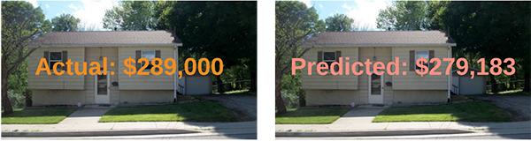
[INFO] avg. house price: $533,388.27, std house price: $493,403.08

[INFO] mean: 27.52%, std: 22.19%

我们的平均绝对百分比误差开始时非常高，但在整个训练过程中继续下降。 在训练结束时，我们在测试集上获得了 27.52% 的平均绝对百分比误差，这意味着，平均而言，我们的网络在其房价预测中将降低约 26-27%。

文末有福利领取哦~

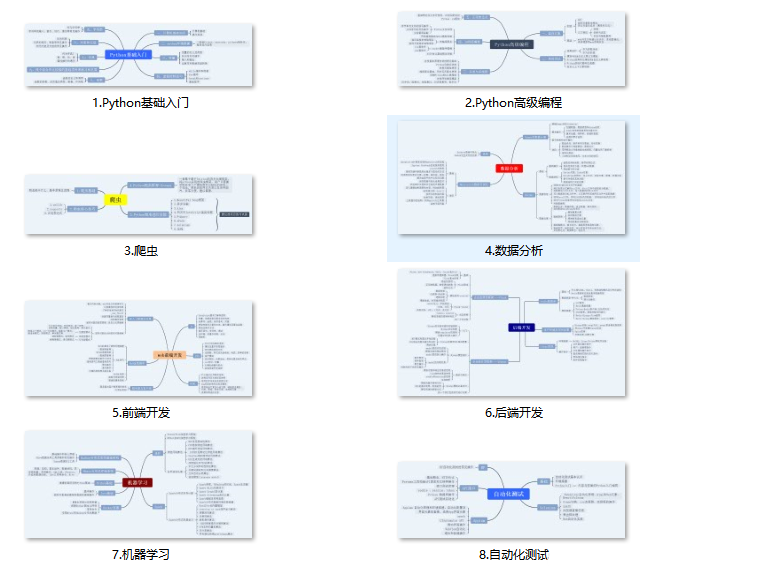
👉一、Python所有方向的学习路线

Python所有方向的技术点做的整理，形成各个领域的知识点汇总，它的用处就在于，你可以按照上面的知识点去找对应的学习资源，保证自己学得较为全面。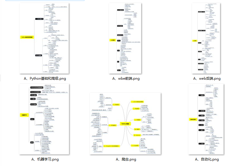

👉二、Python必备开发工具

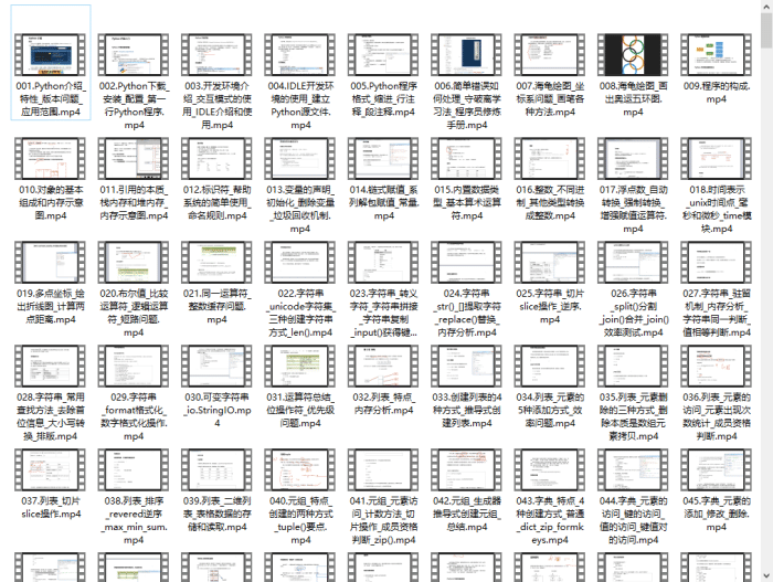
👉三、Python视频合集

观看零基础学习视频，看视频学习是最快捷也是最有效果的方式，跟着视频中老师的思路，从基础到深入，还是很容易入门的。

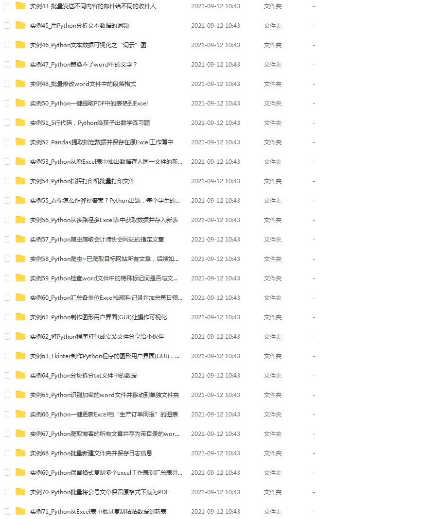
👉 四、实战案例

光学理论是没用的，要学会跟着一起敲，要动手实操，才能将自己的所学运用到实际当中去，这时候可以搞点实战案例来学习。（文末领读者福利）

👉五、Python练习题

检查学习结果。

👉六、面试资料

我们学习Python必然是为了找到高薪的工作，下面这些面试题是来自阿里、腾讯、字节等一线互联网大厂最新的面试资料，并且有阿里大佬给出了权威的解答，刷完这一套面试资料相信大家都能找到满意的工作。

👉因篇幅有限，仅展示部分资料，这份完整版的Python全套学习资料已经上传

网上学习资料一大堆，但如果学到的知识不成体系，遇到问题时只是浅尝辄止，不再深入研究，那么很难做到真正的技术提升。

需要这份系统化的资料的朋友，可以添加V获取：vip1024c （备注python）

一个人可以走的很快，但一群人才能走的更远！不论你是正从事IT行业的老鸟或是对IT行业感兴趣的新人，都欢迎加入我们的的圈子（技术交流、学习资源、职场吐槽、大厂内推、面试辅导），让我们一起学习成长！
59f21623d9efafa68.png)

👉 四、实战案例

光学理论是没用的，要学会跟着一起敲，要动手实操，才能将自己的所学运用到实际当中去，这时候可以搞点实战案例来学习。（文末领读者福利）

👉五、Python练习题

检查学习结果。

👉六、面试资料

我们学习Python必然是为了找到高薪的工作，下面这些面试题是来自阿里、腾讯、字节等一线互联网大厂最新的面试资料，并且有阿里大佬给出了权威的解答，刷完这一套面试资料相信大家都能找到满意的工作。

👉因篇幅有限，仅展示部分资料，这份完整版的Python全套学习资料已经上传

网上学习资料一大堆，但如果学到的知识不成体系，遇到问题时只是浅尝辄止，不再深入研究，那么很难做到真正的技术提升。

需要这份系统化的资料的朋友，可以添加V获取：vip1024c （备注python）
[外链图片转存中…(img-LlRU6qBD-1713090979954)]

一个人可以走的很快，但一群人才能走的更远！不论你是正从事IT行业的老鸟或是对IT行业感兴趣的新人，都欢迎加入我们的的圈子（技术交流、学习资源、职场吐槽、大厂内推、面试辅导），让我们一起学习成长！