Count Vectorizer以及N-Gram模型进行文本特征的向量化表示

学习目标：

1. 学习并理解特征缩放的具体方法：区间缩放+标准化法
2. 理解并使用Count Vectorizer以及N-Gram模型进行文本特征的向量化表示
3. 掌握线性回归和二元多项式回归的基本思想
4. 掌握信息熵与互信息的计算方法
5. 基于上述的基础知识，分别使用Python进行编程练习。

---

学习内容：

1：基于Count Vectorizer特征提取方法与N-Gram模型，使用SKlearn对文档进行向量化表示
2：基于两种特征缩放方法(标准化、区间缩放)，使用SKlearn进行量纲的特征缩放。要求：采用自定义的简单二维数组和IRIS数据集进行实验。
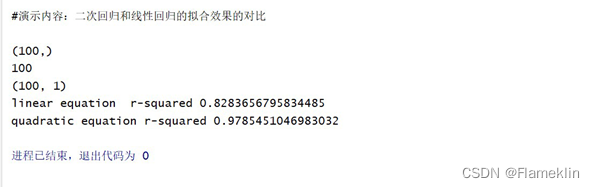
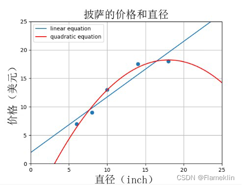
3：使用SKlearn进行线性回归和二次回归曲线的绘制，以及拟合效果的对比(披萨尺寸与价格的回归分析)
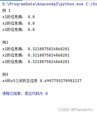
4：信息熵和互信息的计算(数据可自定义)

---

实验步骤及编码：

1：
from sklearn.feature_extraction.text import CountVectorizer
corpus = [
'Jobs was the chairman of Apple Inc., and he was very famous',
'I like to use apple computer',
'And I also like to eat apple'
]

vectorizer =CountVectorizer()
print(vectorizer.fit_transform(corpus).todense())
print(vectorizer.vocabulary_)
print(" ")

import nltk
nltk.download('stopwords')
stopwords = nltk.corpus.stopwords.words('english')
print (stopwords)
print(" ")
vectorizer =CountVectorizer(stop_words='english')
print("after stopwords removal:  ", vectorizer.fit_transform(corpus).todense())
print("after stopwords removal:  ", vectorizer.vocabulary_)
print(" ")
#采用ngram模式进行文档向量化
vectorizer =CountVectorizer(ngram_range=(1,2))
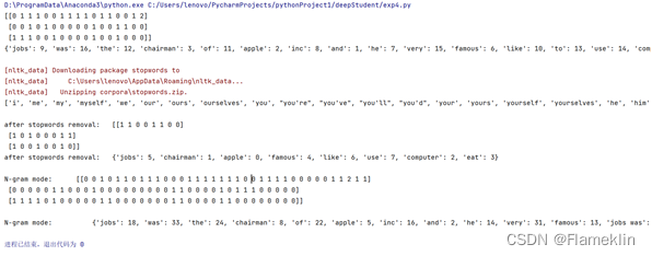
print("N-gram mode:     ",vectorizer.fit_transform(corpus).todense())
print(" ")
print("N-gram mode:         ",vectorizer.vocabulary_)

结果

from sklearn import preprocessing
import numpy as np

X = np.array([[0, 0],
        [0, 0],
        [100, 1],
        [1, 1]])
X_mean = X.mean(axis=0)
X_std = X.std(axis=0)  
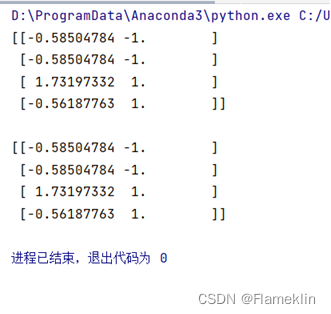
X1 = (X-X_mean)/X_std
print (X1)
print ("")
X_scale = preprocessing.scale(X)
print (X_scale)

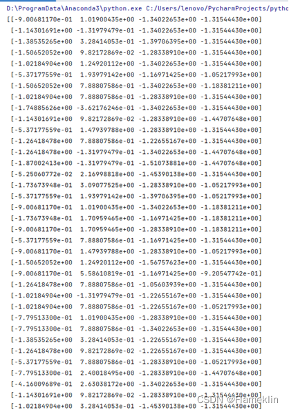
from sklearn import datasets, preprocessing

iris = datasets.load_iris()
X_scale = preprocessing.scale(iris.data)
print (X_scale)
from sklearn.preprocessing import MinMaxScaler

data = [[0, 0],
        [0, 0],
        [100, 1],
        [1, 1]]

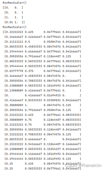
scaler = MinMaxScaler()
print(scaler.fit(data))
print(scaler.transform(data))

from sklearn.preprocessing import MinMaxScaler
data = iris.data
scaler = MinMaxScaler()
print(scaler.fit(data))
print(scaler.transform(data))

3：

print(__doc__)

import numpy as np
import matplotlib.pyplot as plt
from sklearn.linear_model import LinearRegression
from sklearn.preprocessing import PolynomialFeatures
from matplotlib.font_manager import FontProperties

font_set = FontProperties(fname=r"c:\windows\fonts\simsun.ttc", size=20)


def runplt():
    plt.figure()
    plt.title(u'披萨的价格和直径', fontproperties=font_set)
    plt.xlabel(u'直径（inch）', fontproperties=font_set)
    plt.ylabel(u'价格（美元）', fontproperties=font_set)
    plt.axis([0, 25, 0, 25])
    plt.grid(True)
    return plt


X_train = [[6], [8], [10], [14], [18]]
y_train = [[7], [9], [13], [17.5], [18]]
X_test = [[7], [9], [11], [15]]
y_test = [[8], [12], [15], [18]]


plt1 = runplt()
plt1.scatter(X_train, y_train, s=40)

xx = np.linspace(0, 26, 5)
regressor = LinearRegression()
regressor.fit(X_train, y_train)
yy = regressor.predict(xx.reshape(xx.shape[0], 1))

plt.plot(xx, yy, label="linear equation")

quadratic_featurizer = PolynomialFeatures(degree=2)
X_train_quadratic = quadratic_featurizer.fit_transform(X_train)

regressor_quadratic = LinearRegression()
regressor_quadratic.fit(X_train_quadratic, y_train)

xx = np.linspace(0, 26, 100)
print(xx.shape)  # (100,)
print(xx.shape[0])  # 100
xx_quadratic = quadratic_featurizer.transform(xx.reshape(xx.shape[0], 1))
print(xx.reshape(xx.shape[0], 1).shape)  # (100,1)

plt.plot(xx, regressor_quadratic.predict(xx_quadratic), 'r-', label="quadratic equation")
plt.legend(loc='upper left')
plt.show()

X_test_quadratic = quadratic_featurizer.transform(X_test)
print('linear equation  r-squared', regressor.score(X_test, y_test))
print('quadratic equation r-squared', regressor_quadratic.score(X_test_quadratic, y_test))

4
import  numpy as np
from math import log
print("例 1")
def calc_ent(x):
    ent = 0.0
    for p in x:
        end = p* np.log(p)
    return ent
x1=np.array([0.4,0.2,0.2,0.2])
x2=np.array([1])
x3=np.array([0.2,0.2,0.2,0.2])
print("x1的信息熵：",calc_ent(x1))
print("x2的信息熵：",calc_ent(x2))
print("x3的信息熵：",calc_ent(x3))
print("")

print("例2")
def calcShannoEnt(dataSet):
    length, dataDict=float(len(dataSet)),{}
    for data in dataSet:
        try:dataDict[data]+=1
        except:dataDict[data] =1
        return sum([-d/length*log(d/length) for  d in  list(dataDict.values())])
print("x1的信息熵：",calcShannoEnt(['A','B','C','D','A']))
print("x2的信息熵：",calcShannoEnt(['A','A','A','A','A']))
print("x3的信息熵：",calcShannoEnt(['A','B','C','D','E']))

print("")
print("例3")
Ent_x4=calcShannoEnt(['3','4','5','5','3','2','2','6','6','1'])
Ent_x5=calcShannoEnt(['7','2','1','3','2','8','9','1','2','0'])
Ent_x4x5=calcShannoEnt(['37','42','51','53','32','28','29','61','62','10'])
MI_x4_x5=Ent_x4+Ent_x5+Ent_x4x5
print("x4和x5之间的互信息",MI_x4_x5)

---