


特征选取
相关性分析
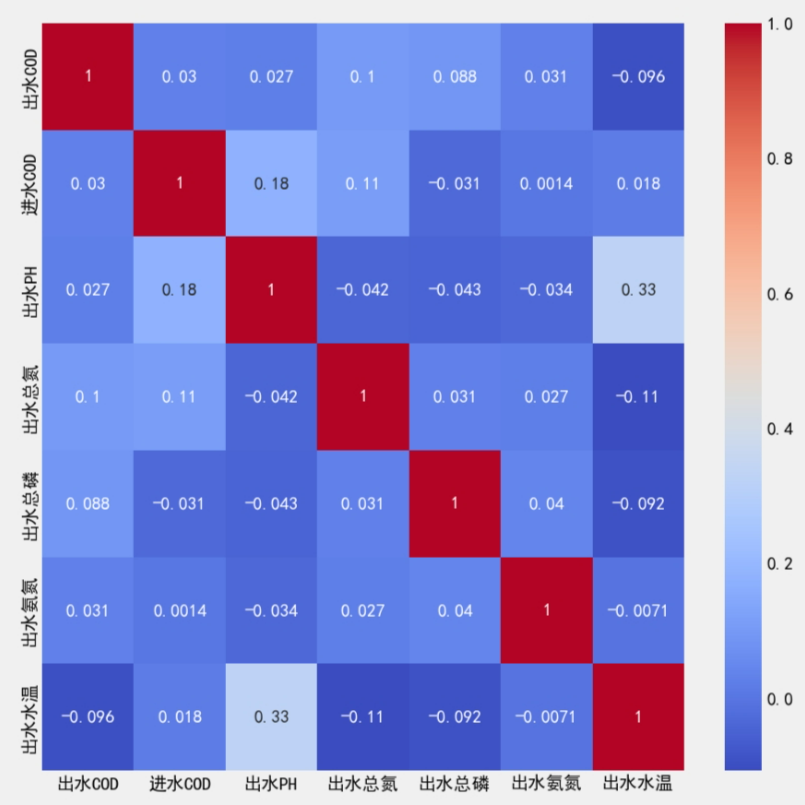
为了对站点出水COD在未来24小时数值做出精准预测,对已有数据特征进行特征筛选,计算目标特征与其他特征的皮尔逊相关指数进行相关性分析.
data= pd.read_csv('data.csv')
data['DateTime'] = pd.to_datetime(data['DateTime'])
data.set_index('DateTime', inplace=True)
# 计算相关矩阵
corr_matrix = data.corr()
plt.figure(figsize=(10,10))
# 绘制热力图
sns.heatmap(corr_matrix, annot=True, cmap='coolwarm')
plt.show()
| 出水总氮 | 出水总磷 | 出水水温 | 出水氨氮 | 进水COD | 出水PH | |
|---|---|---|---|---|---|---|
| 皮尔逊相关性指数 | 0.1 | 0.088 | -0.096 | 0.031 | 0.03 | 0.027 |
Lasso回归
Lasso回归通过L1正则化,将一些不重要的特征权重缩小到0,从而实现特征选择。
# LassoCV 自动调节正则化参数
lasso = LassoCV(cv=5)
lasso.fit(X, y)

# 筛选重要特征
importance = abs(lasso.coef_)
selected_features = X.columns[importance > 0]
print(selected_features)
| 权重不为0的特征 | 进水COD | 出水总氮 | 出水水温 |
|---|
随机森林特征重要度分析
随机森林树模型可以自动计算特征的重要性。
通过随机森林模型对特征进行重要程度分析,得出特征的重要程度
from sklearn.ensemble import RandomForestRegressor

# 训练随机森林模型
model = RandomForestRegressor()
model.fit(X, y)

# 获取特征重要性
importance = model.feature_importances_

# 筛选重要特征
selected_features = X.columns[importance > 0.01]  # 设置阈值
print(selected_features)
| 进水COD | 出水总氮 | 出水PH | 出水氨氮 | 出水水温 | 出水总磷 | |
|---|---|---|---|---|---|---|
| 特征重要程度 | 0.27801 | 0.21714 | 0.14978 | 0.14100 | 0.12185 | 0.09221 |
总结
由以上数据实验分析,决定将出水总磷,和出水PH特征进行删除。
特征工程
标准化
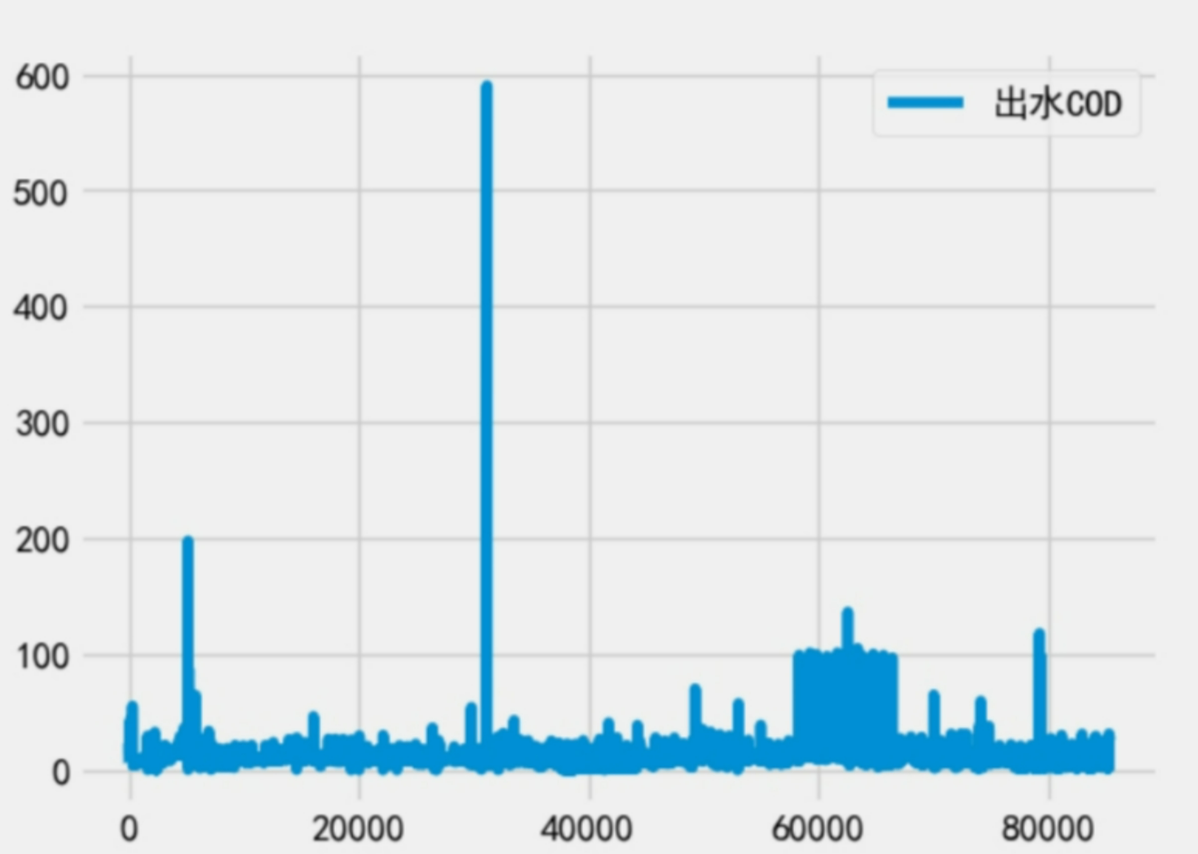
离群值处理
离群值可以通过聚类,也可以通过简单的IQR进行替换
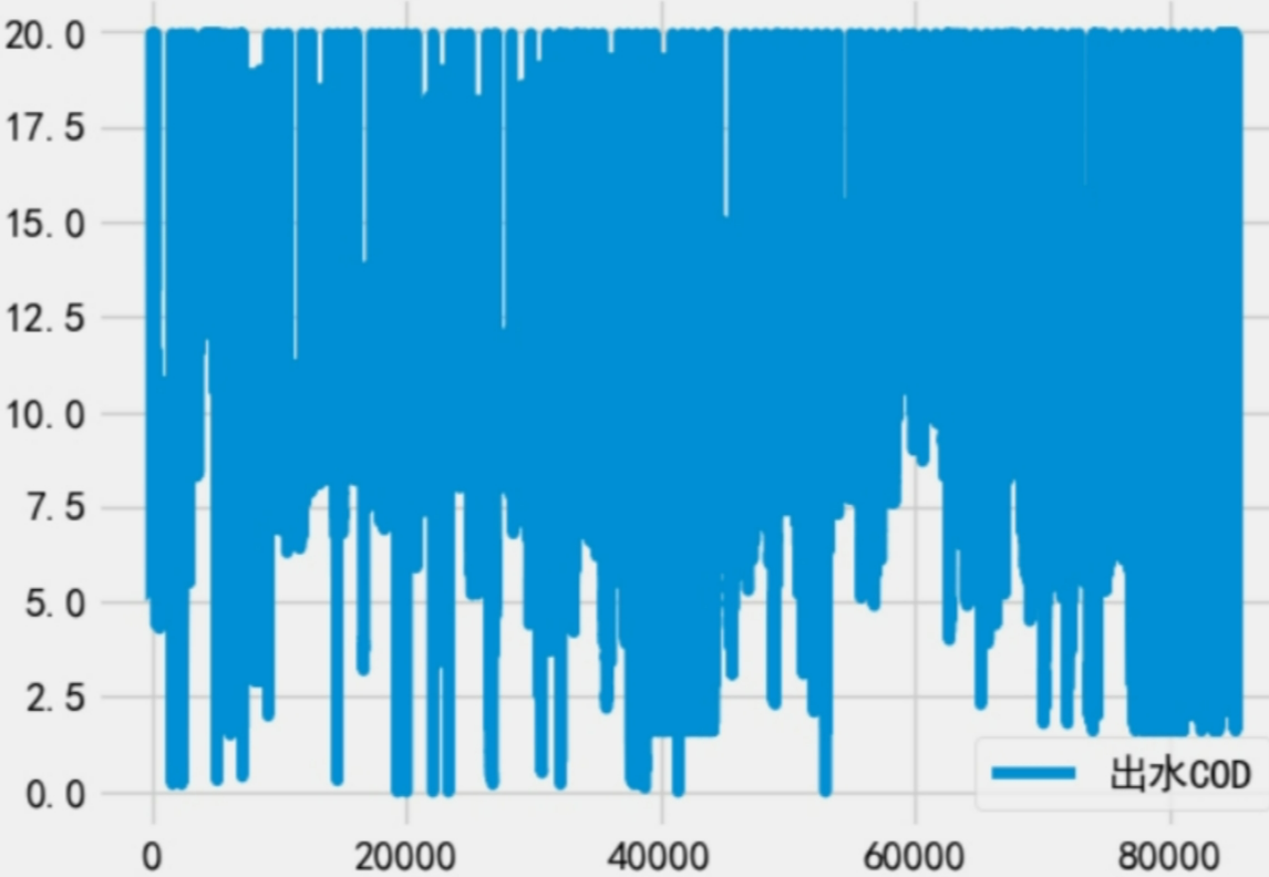
Q1 = data.quantile(0.2)
Q3 = data.quantile(0.80)
IQR = Q3 - Q1
# 将超出IQR范围的值限制在该范围内
data=data.clip(lower=Q1 - 1.5 * IQR, upper=Q3 + 1.5 * IQR, axis=1)
数据处理前图像:
- 折线图
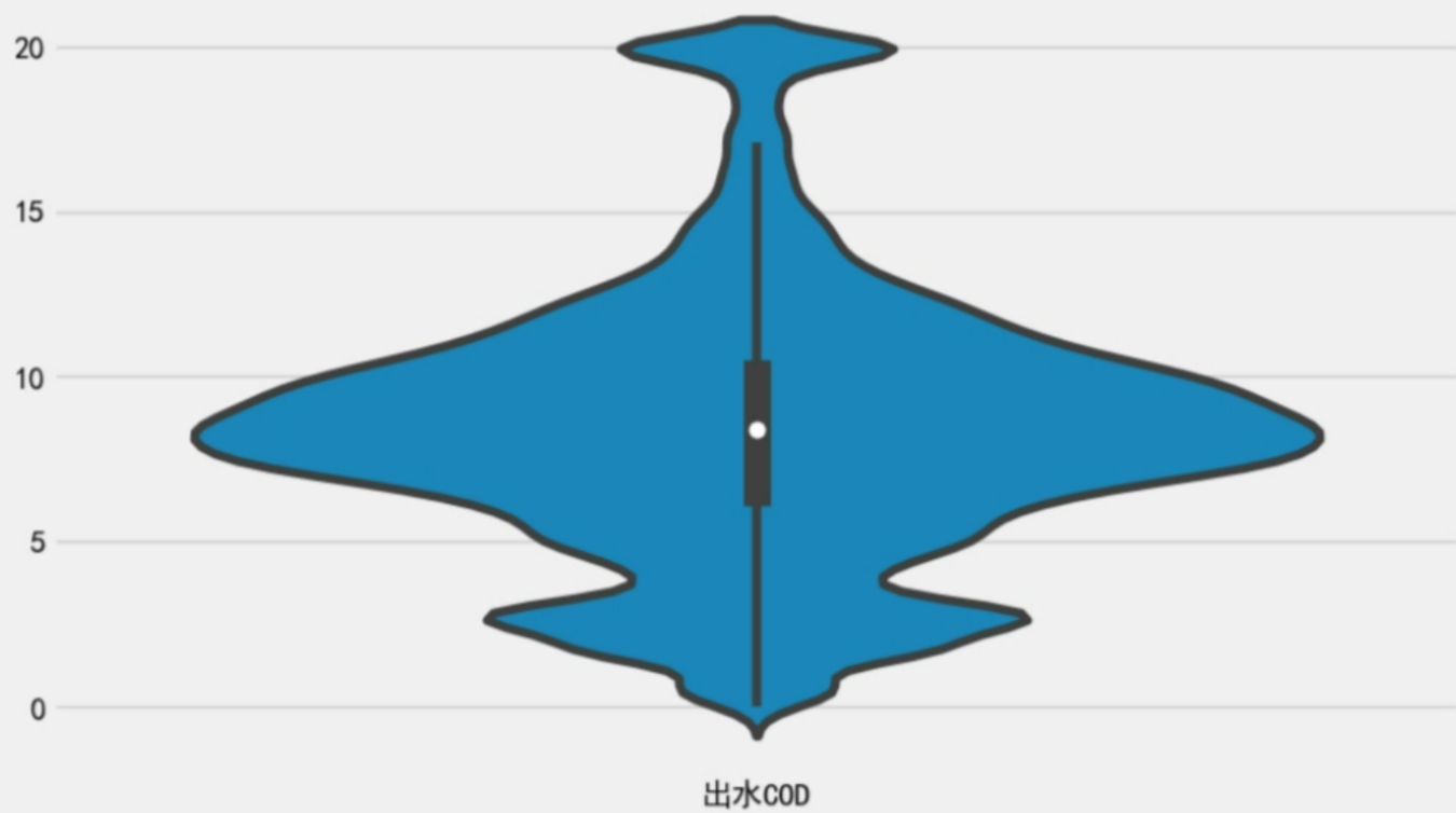
- 小提琴图:

使用IQR五分位距法处理后:
缺失值处理
缺失值占比不大使用KNN算法进行缺失值填补,如果缺失值占比较大,在神经网络模型中可以使用masking方法
data= pd.read_csv('data.csv')
data['DateTime'] = pd.to_datetime(data['DateTime'])
data.set_index('DateTime', inplace=True)

print(data.isnull().sum())

# 使用KNNImputer进行缺失值填补
imputer = KNNImputer(n_neighbors=5)  # 可以调整 n_neighbors 参数
data_filled = pd.DataFrame(imputer.fit_transform(data), columns=data.columns, index=data.index)

print("填补后缺失值:\n", data_filled.isnull().sum())
print(data_filled.head())

时间窗口大小确定
- 通过简单的BP神经网络,对不同大小的时间窗口数据集进行训练测试,找出最适合的窗口大小
- 历史两天的数据作为输入
- 历史一周的数据作为输入
- 历史两周的数据作为输入
| 输入维度 | MAE | MSE |
|---|---|---|
| 2*24 | 0.0925 | 0.0202 |
| 7*24 | 0.0891 | 0.0195 |
| 14*24 | 0.0882 | 0.0192 |
通过比较,224作为模型输入效果最差,724和1424作为模型输入效果相差不大,为了减小模型的参数复杂度,选择724作为模型的输入,窗口大小为7
# BP神经网络
model_bp = Sequential()
model_bp.add(Flatten(input_shape=(window_size, X.shape[2])))
model_bp.add(Dense(32, activation='relu', kernel_regularizer=l2(0.001)))
model_bp.add(Dense(64, activation='relu', kernel_regularizer=l2(0.001)))
model_bp.add(Dense(128, activation='relu', kernel_regularizer=l2(0.001)))
model_bp.add(Dropout(0.1)) # Dropout层,丢弃30%的神经元
model_bp.add(Dense(128, activation='relu', kernel_regularizer=l2(0.001)))
model_bp.add(Dropout(0.5))
model_bp.add(Dense(64, activation='relu', kernel_regularizer=l2(0.001)))
model_bp.add(Dropout(0.3))
model_bp.add(Dense(32, activation='relu', kernel_regularizer=l2(0.001)))
model_bp.add(Dropout(0.3))
model_bp.add(Dense(forecast_size, activation='linear'))
model_bp.compile(optimizer='adam', loss='mse', metrics=['mae'])
reduce_lr = ReduceLROnPlateau(monitor='val_loss', factor=0.5, patience=3, min_lr=0.00001)
history_bp = model_bp.fit(X_train, y_train, validation_data=(X_val, y_val),
epochs=50, batch_size=32, callbacks=[reduce_lr])
import matplotlib.pyplot as plt
model_bp.evaluate(X_test, y_test)
predictions = model_bp.predict(X_test)
print(y_test)
print(predictions)
# y_test = y_test.reshape(-1,1)
# predictions = predictions.reshape(-1,1)
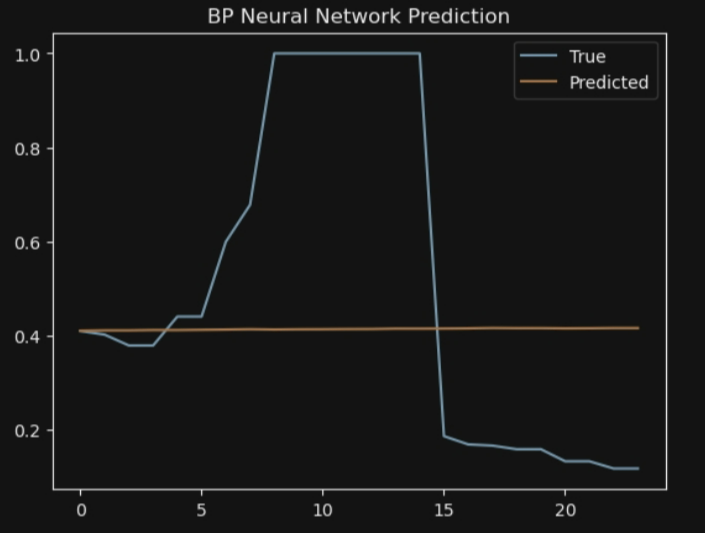
plt.plot(y_test[1], label='True')
plt.plot(predictions[1] ,label='Predicted')
plt.title('BP Neural Network Prediction')
plt.legend()
plt.show()
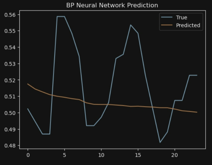
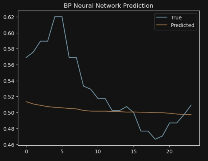
plt.plot(y_test[0], label='True')
plt.plot(predictions[0] ,label='Predicted')
plt.title('BP Neural Network Prediction')
plt.legend()
plt.show()
plt.plot(history_bp.history['loss'], label='Train Loss')
plt.plot(history_bp.history['val_loss'], label='Val Loss')
plt.title('BP Neural Network Training Loss')
plt.xlabel('Epochs')
plt.ylabel('Loss')
plt.legend()
plt.show()
mae = mean_absolute_error(y_test, predictions)
mse = mean_squared_error(y_test, predictions)
are = np.mean(np.abs((y_test - predictions) / y_test)) * 100 # 以百分比表示
print(f'MAE: {mae:.4f}')
print(f'MSE: {mse:.4f}')
print(f'ARE: {are:.2f}%')
模型建立
目标,根据已有数据建立并训练模型,使用历史7天的数据,对任意时刻未来24小时后的数据进行预测
LSTM
# 优化后的LSTM模型
model_lstm = Sequential()
model_lstm.add(LSTM(64, return_sequences=True, input_shape=(window_size, X.shape[2]),
kernel_regularizer=l2(0.001))) # 添加L2正则化
model_lstm.add(Dropout(0.3)) # 添加Dropout层
model_lstm.add(LSTM(64, kernel_regularizer=l2(0.001))) # 第二层LSTM,同样添加正则化
model_lstm.add(Dropout(0.3)) # 再次添加Dropout层
model_lstm.add(Dense(forecast_size, activation='linear'))
model_lstm.compile(optimizer='adam', loss='mse', metrics=['mae'])
# 定义学习率调度器和早停回调
reduce_lr = ReduceLROnPlateau(monitor='val_loss', factor=0.5, patience=5, min_lr=0.00001)
early_stopping = EarlyStopping(monitor='val_loss', patience=10, restore_best_weights=True)
history_lstm = model_lstm.fit(X_train, y_train, validation_data=(X_val, y_val),
epochs=50, batch_size=32,
callbacks=[reduce_lr, early_stopping])
model_lstm.evaluate(X_test, y_test)
import matplotlib.pyplot as plt
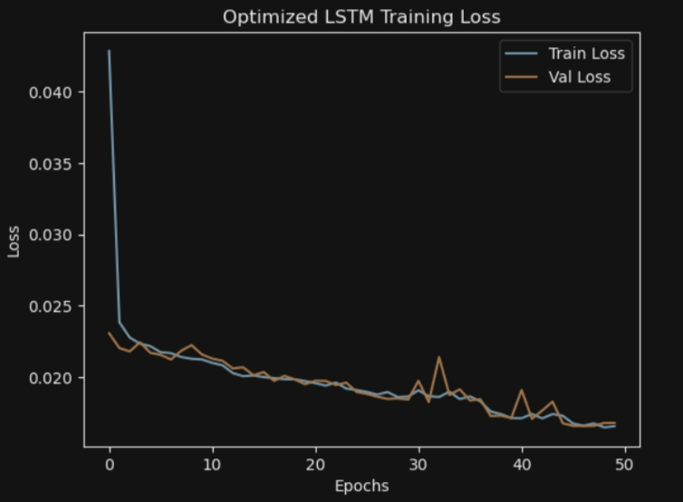
plt.plot(history_lstm.history['loss'], label='Train Loss')
plt.plot(history_lstm.history['val_loss'], label='Val Loss')
plt.title('Optimized LSTM Training Loss')
plt.xlabel('Epochs')
plt.ylabel('Loss')
plt.legend()
plt.show()
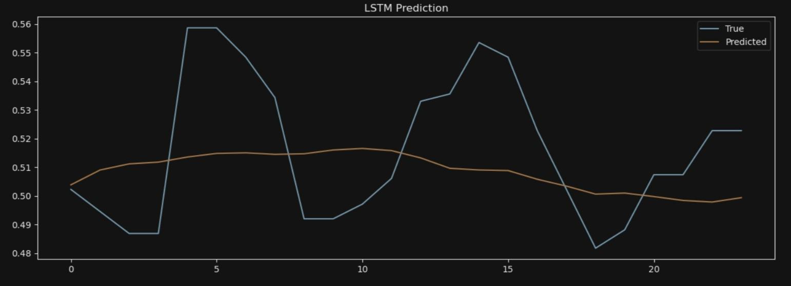
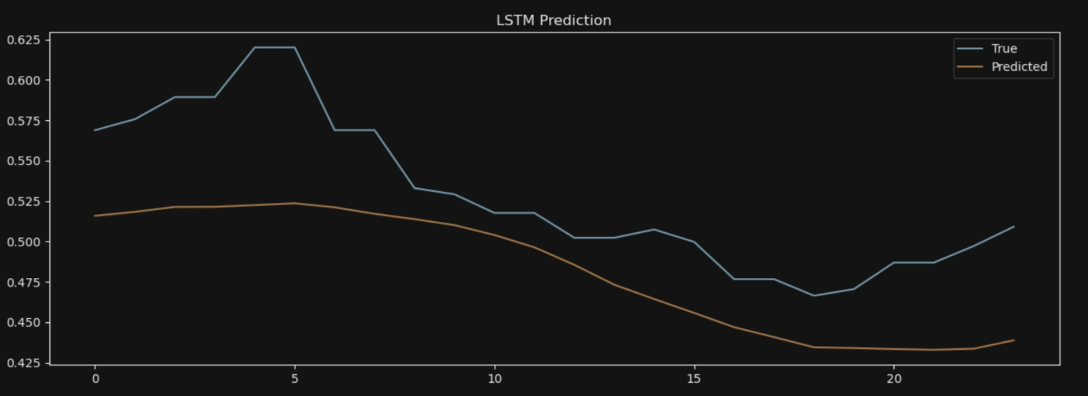
predictions = model_lstm.predict(X_test)
plt.figure(figsize=(15, 5))
plt.plot(y_test[0], label='True')
plt.plot(predictions[0], label='Predicted')
plt.title('LSTM Prediction')
plt.legend()
plt.show()
7*24:
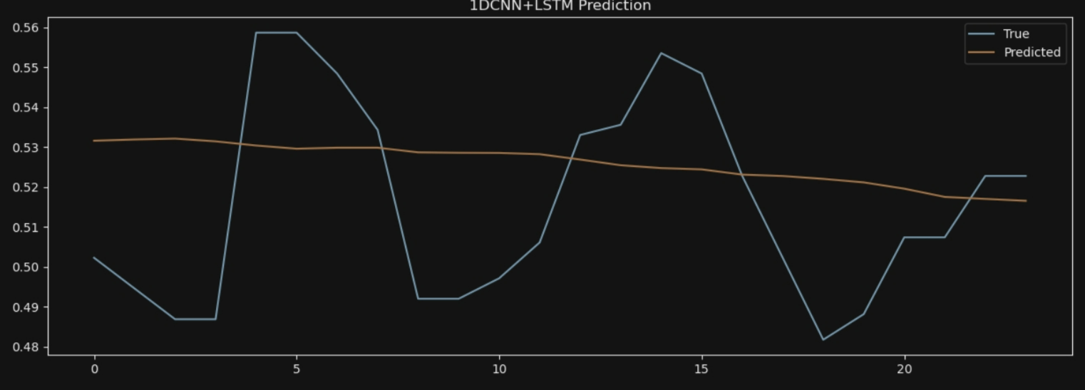
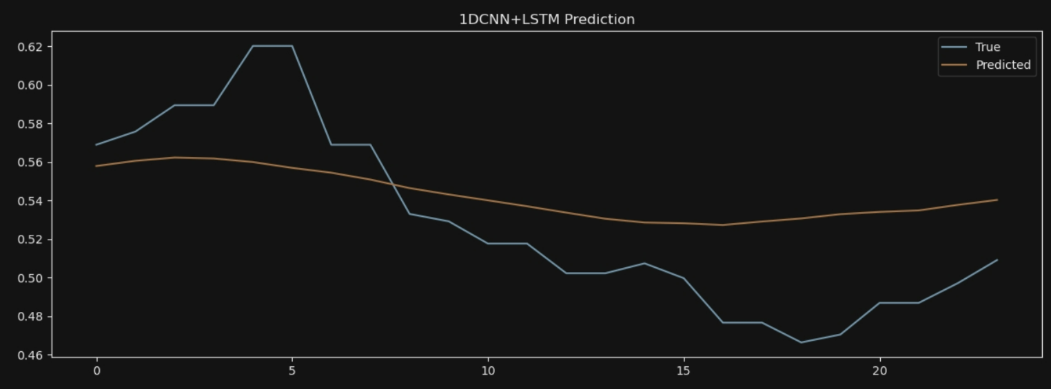
1D-CNN+LSTM

#1D CNN+LSTM
model_cnn_lstm = Sequential()
model_cnn_lstm.add(Conv1D(64, kernel_size=3, activation='relu', input_shape=(window_size, X.shape[2]),
kernel_regularizer=l2(0.001))) # 添加L2正则化
model_cnn_lstm.add(MaxPooling1D(pool_size=2))
model_cnn_lstm.add(Dropout(0.5)) # 添加Dropout层
model_cnn_lstm.add(LSTM(64, kernel_regularizer=l2(0.001))) # LSTM层,同样添加正则化
model_cnn_lstm.add(Dropout(0.5)) # 再次添加Dropout层
model_cnn_lstm.add(Dense(forecast_size, activation='linear'))
model_cnn_lstm.compile(optimizer='adam', loss='mse', metrics=['mae'])
reduce_lr = ReduceLROnPlateau(monitor='val_loss', factor=0.5, patience=5, min_lr=0.00001)
early_stopping = EarlyStopping(monitor='val_loss', patience=10, restore_best_weights=True)
history_cnn_lstm = model_cnn_lstm.fit(X_train, y_train, validation_data=(X_val, y_val),
epochs=50, batch_size=32,
callbacks=[reduce_lr, early_stopping])
model_cnn_lstm.evaluate(X_test, y_test)
import matplotlib.pyplot as plt
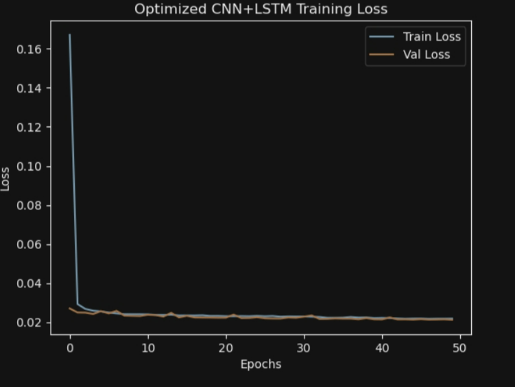
plt.plot(history_cnn_lstm.history['loss'], label='Train Loss')
plt.plot(history_cnn_lstm.history['val_loss'], label='Val Loss')
plt.title('Optimized CNN+LSTM Training Loss')
plt.xlabel('Epochs')
plt.ylabel('Loss')
plt.legend()
plt.show()
predictions = model_cnn_lstm.predict(X_test)
plt.figure(figsize=(15, 5))
plt.plot(y_test[1], label='True')
plt.plot(predictions[1], label='Predicted')
plt.title('1DCNN+LSTM Prediction')
plt.legend()
plt.show()
plt.figure(figsize=(15, 5))
plt.plot(y_test[0], label='True')
plt.plot(predictions[0], label='Predicted')
plt.title('1DCNN+LSTM Prediction')
plt.legend()
plt.show()
mae = mean_absolute_error(y_test, predictions)
mse = mean_squared_error(y_test, predictions)
are = np.mean(np.abs((y_test - predictions) / y_test)) * 100 # 以百分比表示
print(f'MAE: {mae:.4f}')
print(f'MSE: {mse:.4f}')
7*24:
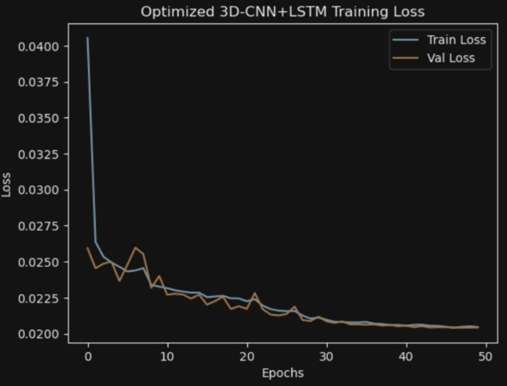
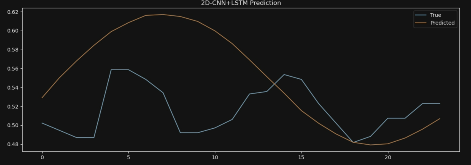
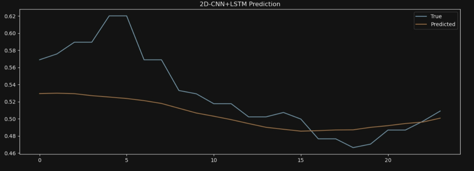
2D-CNN+LSTM
# 调整数据形状
X_train_2d = X_train.reshape(-1, window_size, X.shape[2], 1)
X_val_2d = X_val.reshape(-1, window_size, X.shape[2], 1)
X_test_2d = X_test.reshape(-1, window_size, X.shape[2], 1)

model_2dcnn_lstm = Sequential()
model_2dcnn_lstm.add(Conv2D(64, kernel_size=(3, 3), activation='relu', input_shape=(window_size, X.shape[2], 1),
                            kernel_regularizer=l2(0.001)))  # 添加L2正则化
model_2dcnn_lstm.add(MaxPooling2D(pool_size=(2, 2)))
model_2dcnn_lstm.add(Dropout(0.3))  # 添加Dropout层

# Reshape用于将卷积层的输出调整为LSTM层可以接受的形状
model_2dcnn_lstm.add(Reshape((model_2dcnn_lstm.layers[-1].output_shape[1] * model_2dcnn_lstm.layers[-1].output_shape[2],
                             model_2dcnn_lstm.layers[-1].output_shape[-1])))

model_2dcnn_lstm.add(LSTM(64, kernel_regularizer=l2(0.001)))  # LSTM层,添加L2正则化
model_2dcnn_lstm.add(Dropout(0.3))  # 再次添加Dropout层
model_2dcnn_lstm.add(Dense(forecast_size, activation='linear'))

model_2dcnn_lstm.compile(optimizer='adam', loss='mse', metrics=['mae'])

# 定义学习率调度器和早停回调
reduce_lr = ReduceLROnPlateau(monitor='val_loss', factor=0.5, patience=5, min_lr=0.00001)
early_stopping = EarlyStopping(monitor='val_loss', patience=10, restore_best_weights=True)

# 训练模型
history_2dcnn_lstm = model_2dcnn_lstm.fit(X_train_2d, y_train, validation_data=(X_val_2d, y_val),
                                          epochs=50, batch_size=32,
                                          callbacks=[reduce_lr, early_stopping])

# 模型评估和预测
model_2dcnn_lstm.evaluate(X_test_2d, y_test)

# 可视化训练过程中的损失变化
import matplotlib.pyplot as plt

plt.plot(history_2dcnn_lstm.history['loss'], label='Train Loss')
plt.plot(history_2dcnn_lstm.history['val_loss'], label='Val Loss')
plt.title('Optimized 3D-CNN+LSTM Training Loss')
plt.xlabel('Epochs')
plt.ylabel('Loss')
plt.legend()
plt.show()

# 预测并可视化
predictions = model_2dcnn_lstm.predict(X_test_2d)

plt.figure(figsize=(15, 5))
plt.plot(y_test[0], label='True')
plt.plot(predictions[0], label='Predicted')
plt.title('3D-CNN+LSTM Prediction')
plt.legend()
plt.show()
7*24:
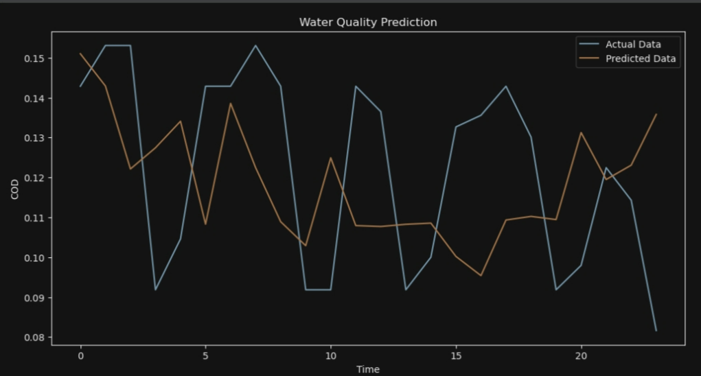
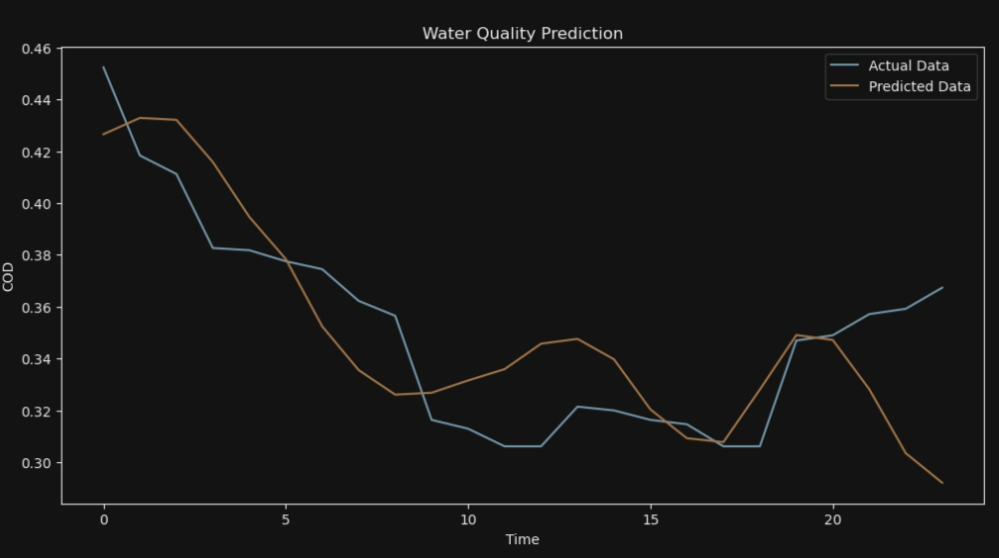
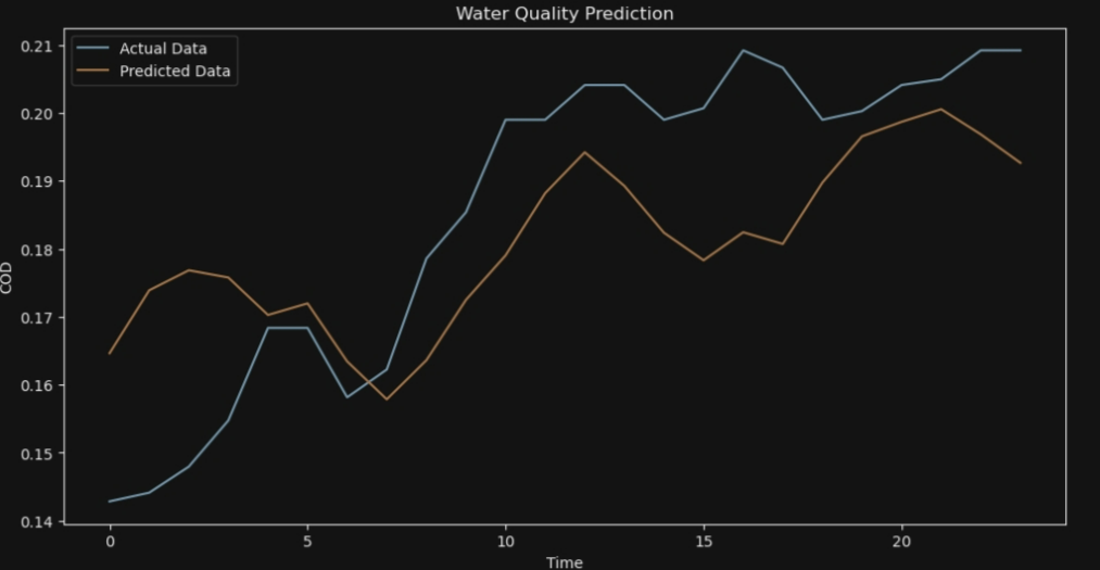
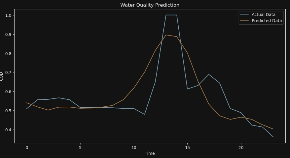
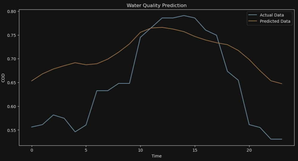
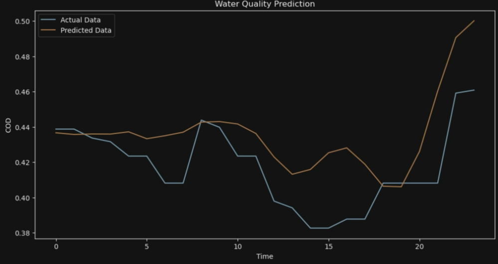
HMM-Bi-LSTM
# 使用HMM进行数据降维
n_components = 7  # HMM的状态数量,可以根据需要调整
hmm_model = GaussianHMM(n_components=n_components, covariance_type="diag", n_iter=1000, random_state=42)

scaler = StandardScaler()
data_scaled_std = scaler.fit_transform(data_x)
joblib.dump(scaler, 'scaler_hmm.gz')

print(data_scaled_std.shape)
hmm_model.fit(data_scaled_std)

hmm_features = hmm_model.predict_proba(data_scaled_std)

X_hmm = []
for i in range(window_size, len(hmm_features) - forecast_size):
    X_hmm.append(hmm_features[i - window_size:i])
X_hmm = np.array(X_hmm)


def build_bilstm_model(input_shape, forecast_size):
    model = Sequential()
    model.add(Bidirectional(LSTM(64, return_sequences=True), input_shape=input_shape))
    model.add(Bidirectional(LSTM(32)))
    model.add(Dense(forecast_size))
    model.compile(optimizer='adam', loss='mse', metrics=['mae', are_metric])
    return model

# 构建BiLSTM模型
input_shape = (window_size, n_components)
bilstm_model = build_bilstm_model(input_shape, forecast_size)

# 拆分数据集
X_train_hmm, X_temp_hmm, y_train, y_temp = train_test_split(X_hmm, Y, test_size=0.3, random_state=42)
X_val_hmm, X_test_hmm, y_val, y_test = train_test_split(X_temp_hmm, y_temp, test_size=0.5, random_state=42)

print(X_train_hmm.shape, y_train.shape)
reduce_lr = ReduceLROnPlateau(monitor='val_loss', factor=0.5, patience=5, min_lr=0.00001)

# 训练BiLSTM模型
history = bilstm_model.fit(X_train_hmm, y_train, epochs=120, batch_size=32, validation_data=(X_val_hmm, y_val),callbacks=[reduce_lr])


# 评估模型
loss, mae, are = bilstm_model.evaluate(X_test_hmm, y_test)
print(f"Test Loss: {loss}, Test MAE: {mae}, Test ARE: {are}")

import matplotlib.pyplot as plt

# 进行预测
y_pred = bilstm_model.predict(X_test_hmm)


for i in range (10):
    # 可视化结果
    plt.figure(figsize=(12, 6))
    plt.plot(y_test[i], label='Actual Data')
    plt.plot(y_pred[i], label='Predicted Data')
    plt.legend()
    plt.xlabel('Time')
    plt.ylabel('COD')
    plt.title('Water Quality Prediction')
    plt.show()
7*24
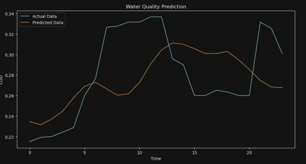
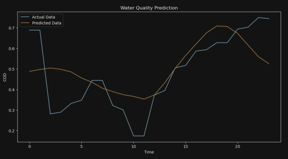
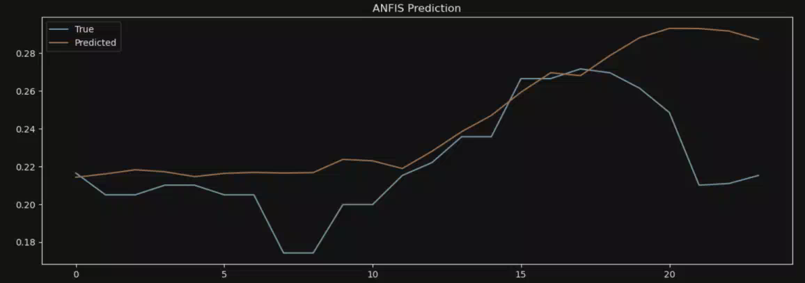
ANFIS
class ANFISLayer(tf.keras.layers.Layer):
    def __init__(self, num_rules, num_features):
        super(ANFISLayer, self).__init__()
        self.num_rules = num_rules
        self.num_features = num_features
        self.mfs = []
        for i in range(num_rules):
            self.mfs.append([self.add_weight(shape=(1,), initializer="random_normal", trainable=True)
                             for _ in range(num_features)])
        self.bias = self.add_weight(shape=(num_rules,), initializer="random_normal", trainable=True)

    def call(self, inputs):
        rules_out = []
        for i in range(self.num_rules):
            rule = 1
            for j in range(self.num_features):
                rule *= tf.exp(-tf.square(inputs[:, j] - self.mfs[i][j]))  # 模糊隶属度函数
            rules_out.append(rule)
        rules_out = tf.stack(rules_out, axis=-1) + self.bias
        return rules_out

# 搭建ANFIS模型
def build_anfis_model(input_shape, num_rules=3):
    model = Sequential()
    model.add(ANFISLayer(num_rules=num_rules, num_features=input_shape[-1]))
    model.add(Dense(64, activation='relu'))
    model.add(Bidirectional(LSTM(64, return_sequences=True)))
    model.add(Bidirectional(LSTM(64)))
    model.add(Dense(forecast_size))
    model.compile(optimizer='adam', loss='mse', metrics=['mae', are_metric])
    return model

input_shape = X_train.shape[1:]

anfis_model = build_anfis_model(input_shape)

anfis_model.build(input_shape=(None, *input_shape))

anfis_model.summary()

reduce_lr = ReduceLROnPlateau(monitor='val_loss', factor=0.5, patience=3, min_lr=0.00001)

history = anfis_model.fit(X_train, y_train, validation_data=(X_val, y_val), epochs=50, batch_size=12, callbacks=[reduce_lr])

test_loss, test_mae, test_are = anfis_model.evaluate(X_test, y_test)
print(f'Test Loss: {test_loss:.4f}')
print(f'Test MAE: {test_mae:.4f}')
print(f'Test ARE: {test_are:.2f}%')

predictions = anfis_model.predict(X_test)

import matplotlib.pyplot as plt

plt.plot(history.history['loss'], label='Train Loss')
plt.plot(history.history['val_loss'], label='Val Loss')
plt.title('Optimized ANFIS Training Loss')
plt.xlabel('Epochs')
plt.ylabel('Loss')
plt.legend()
plt.show()

for i in range(10,20):
    plt.figure(figsize=(15, 5))
    plt.plot(y_test[i], label='True')
    plt.plot(predictions[i], label='Predicted')
    plt.title('ANFIS Prediction')
    plt.legend()
    plt.show()
7*24
总结
| MAE | MSE | ARE | |
|---|---|---|---|
| LSTM | 0.1068 | 0.0240 | |
| 1D-CNN+LSTM | 0.0891 | 0.0201 | |
| 2D-CNN+LSTM | 0.0893 | 0.0192 | 39.15% |
| HMM-Bi-LSTM | 0.0973 | 0.0194 | |
| ANFIS | 0.0950 | 0.0201 | 37.79% |
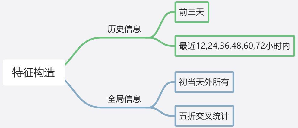
LightGBM
由于机器学习算法不具备自动提取特征的能力 ,输入一般为以二维表格形式表示的特征矩阵,所以需要设计特征添加到数据集中.
特征提取思路:
- 定义一天中的不同时段(
period)。每个时段由一天中的小时数决定,时间范围被分成了8个时段(0-7),每个时段对应一个特定的编号。
- 时段定义:
- 时段 0: 23点、0点、1点
- 时段 1: 2点、3点、4点
- 时段 2: 5点、6点、7点
- 时段 3: 8点、9点、10点、11点
- 时段 4: 12点、13点
- 时段 5: 14点、15点、16点、17点
- 时段 6: 18点
- 时段 7: 19点、20点、21点、22点
- 将时段编号转为独热编码(One-hot Encoding)特征,并将这些特征加入数据集中,删除原来的
period和hour列。
- 历史平移特征
- 将指定列
col的数据向后平移若干时刻,以捕捉历史数据对当前时刻的影响。
- 将指定列
- 差分特征
- 计算指定列的前后时刻差值来捕捉数据的变化趋势,结合平移特征的使用
- 窗口统计特征 12,24,36,48,60,72
- 在一段时间窗口内计算一些统计量(如均值、最大值、最小值、总和和标准差),帮助模型捕捉数据在时间序列中的局部特征
- 全局特征
- 加权平均值
- 五折交叉统计
data = out_COD.resample('H').mean()

"""
经过实验,填充缺失值的效果不如不填充缺失值
"""
data = data.fillna(method='ffill')

#使用one_hot标注数据的时间段
period_dict = {
    23: 0, 0: 0, 1: 0,
    2:1, 3:1, 4:1,
    5: 2, 6: 2, 7: 2,
    8:3, 9:3, 10:3, 11:3,
    12:4, 13:4,
    14: 5, 15: 5, 16: 5, 17: 5,
    18: 6,
    19: 7, 20: 7, 21: 7, 22: 7,
}
# 使用period_dict字典创建新特征列

data['hour'] = data.index.hour
def get_period(hour):
    for key, value in period_dict.items():
        if hour == key:
            return value
data['period'] = data['hour'].apply(get_period)
one_hot_df = pd.get_dummies(data['period'], prefix='type')
data = data.join(one_hot_df)
data = data.drop(['period','hour'], axis=1)
data = data.replace({True: 1, False: 0})

print(data.head())

# 历史平移
for i in range(1, 72):
    data[f'target_shift{i}'] = data[col].shift(i)

# 历史平移 + 差分特征
for i in range(1, 72):
    data[f'diff_{i}'] = data[col].diff(i).shift(1)

# 历史平移 + 窗口统计
for win in [12,24,36,48,60,72]:
    data[f'target_shift10_win{win}_mean'] = data[col].rolling(window=win, min_periods=3,
                                                                                         closed='left').mean().values
    data[f'target_shift10_win{win}_max'] = data[col].rolling(window=win, min_periods=3,
                                                                                        closed='left').max().values
    data[f'target_shift10_win{win}_min'] = data[col].rolling(window=win, min_periods=3,
                                                                                        closed='left').min().values
    data[f'target_shift10_win{win}_sum'] = data[col].rolling(window=win, min_periods=3,
                                                                                        closed='left').sum().values
    data[f'target_shift710win{win}_std'] = data[col].rolling(window=win, min_periods=3,
                                                                                        closed='left').std().values

"""归一化"""
# scaler = MinMaxScaler()
# normalized_features = scaler.fit_transform(data)
# normalized_df = pd.DataFrame(normalized_features, columns=data.columns,index=data.index)
normalized_df = data.dropna()

y = normalized_df[col]
X= normalized_df.drop(col,axis=1)

# 训练集,测试集和验证集切分
trn_x, trn_y = X[X.index < '2024-01-01'], y[X.index < '2024-01-01']
val_x, val_y =  X[(X.index >= '2024-01-01')&(X.index<'2024-05-01')], y[(X.index >= '2024-01-01')&(X.index<'2024-05-01')]
test_x, test_y =  X[X.index>='2024-05-01'], y[X.index>='2024-05-01']


# # 计算每列的IQR
# Q1 = data.quantile(0.25)
# Q3 = data.quantile(0.75)
# IQR = Q3 - Q1
# # 将超出IQR范围的值限制在该范围内
# trn_x=trn_x.clip(lower=Q1 - 1.5 * IQR, upper=Q3 + 1.5 * IQR, axis=1)

# 构建模型输入数据
train_matrix = lgb.Dataset(trn_x, label=trn_y)
valid_matrix = lgb.Dataset(val_x, label=val_y)

lgb_params = {
    'boosting_type': 'rf',
    'objective': 'regression',
    'metric': 'mae',
    'min_child_weight':5 ,
    'num_leaves': 2 **7,
    'lambda_l2': 10,
    'feature_fraction': 0.8,
    'bagging_fraction': 0.8,
    'bagging_freq': 4,
    'learning_rate': 0.05,
    'seed': 2024,
    'nthread': 16,
    'verbose': -1,
}
# 训练模型
model = lgb.train(lgb_params, train_matrix, 5000, valid_sets=[train_matrix, valid_matrix],
                  categorical_feature=[], verbose_eval=50, early_stopping_rounds=50)
# 验证集和测试集结果预测
test_y_pre = model.predict(test_x, num_iteration=model.best_iteration)

model.save_model("LGB_rf_1-72data_out1h.txt")

# 离线分数评估
score = mean_absolute_error(test_y_pre, test_y)
测试集预测结果:
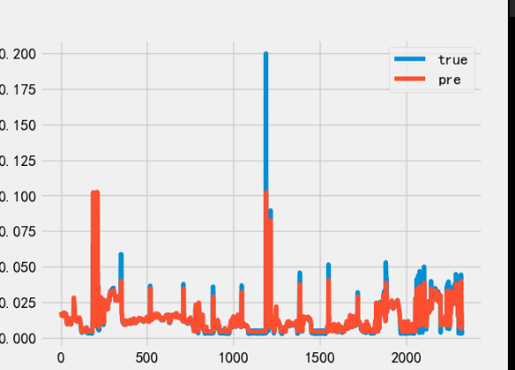
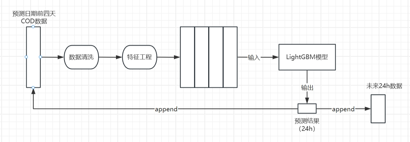
由于LightGBM在做回归任务的时候只能单目标输出,所以该模型的输出是预测未来1h,通过将预测值添加到数据集重新构造数据输入给模型,循环输出24次,以达到预测未来24小时的数据,这样做会使误差累积
 测试集预测:
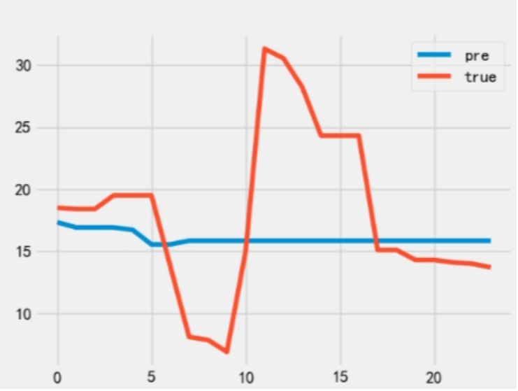
mse 45.06484102310909
mae 4.953343859515587
总结
- 普通神经网络在模型收敛之后能够拟合出一条平滑的曲线,但是对于数据随机性比较强,变化波动较大的数据,不能够很好的拟合出数据的变化趋势
- 机器学习在时间序列预测由于只能单目标输出,所以在预测时间窗口较长的任务时,需要将预测结果迭代预测,造成误差累积,效果不如神经网络
- 为了能够拟合出数据的变化趋势和拨动,可以在神经网络前加模糊推理层,因为模糊推理的隶属度函数需要自己分析所以难度较大,简单的隶属度函数能够描述波动,但是MAE值比较高,对于复杂数据,波动情况效果也比较差
- 使用HMM隐马尔可夫模型,在输入到神经网络之前先对数据的隐含关系进行分析,同样能够很好的拟合出模型的变化趋势,而且模型能够自动捕获数据的信息,相比于ANFIS模型容易训练,切效果较好.


 2321
2321

 被折叠的 条评论
为什么被折叠?
被折叠的 条评论
为什么被折叠?
 到【灌水乐园】发言


