


 本文档是ISE3002课程的学习笔记,涵盖了生产和服务系统的规划概念,包括系统模型、产能规划、预测方法、总量规划、主生产计划、库存管理和控制、物料需求计划、操作调度等内容。讨论了如设计容量、有效容量、时间序列模型、移动平均法、经济订货批量、JIT生产系统、看板系统等关键概念,并强调了合作、库存管理和减少浪费在生产流程中的重要性。
Planning of Production and Service Systems学习笔记
课件引用于香港理工大学ISE3002课程
Content
- Chapter 1: The Systems Concept
- Chapter 2: Capacity Planning
- Chapter 3: Forecasting
-
- Approaches to Forecasting
-
- Qualitative Forecasting Techniques
- Quantitative Forecasting Techniques (Forecasting Models):
- Chapter 4: Aggregate Planning 总体规划
-
- Aggregate Planning V.S. Capacity Planning
- Example 1
- Strategy 1: Chase Strategy
- Strategy 2: Level Strategy
- Strategy 3:
- Strategy 4:
- Example 2
- Methods of Aggregate Planning
- Chapter 5: Master Production Planning – Master Production Schedule (MPS)
- Chapter 6: Inventory Management and Control
- Chapter 7: Material Requirements Planning (MRP)
- Chapter 8: Operations Loading and Scheduling
- Chapter 9: Just-in-Time/Lean Manufacture
-
- 1. Main Purpose of Toyota Production System
- Use of the pull system
- 2. Inventory Hides Problems
- 3. Wastages
- 4. Man-hour reduction
- 5. JIT Layout
- 6. Leveling (Smoothing out) the Production System
- 7. Reduction of Machine Set-up Time
- 8. Shorten the Lead time
- 9. Reduce Inventory
- 10. Zero Inventory as A Challenge
- 11. The "Kanban" System
- 12. JIT Partnership
- 13. Quality Circles
- 14. Implementation of JIT
Chapter 1: The Systems Concept
The Transformational Model of a System
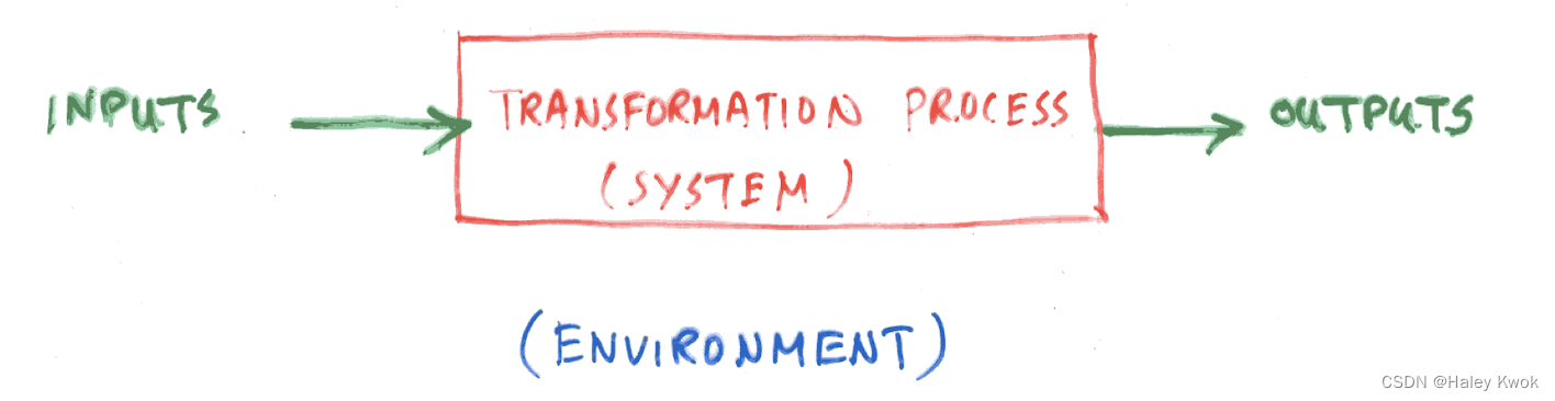
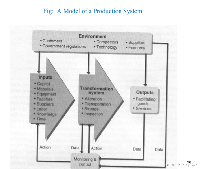
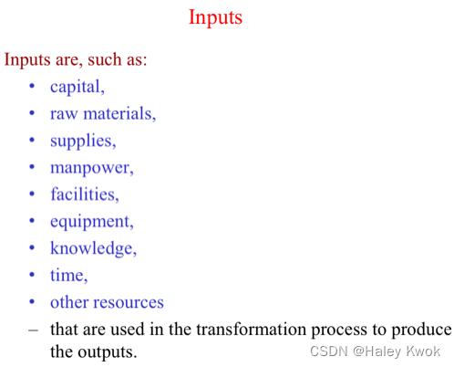
Input
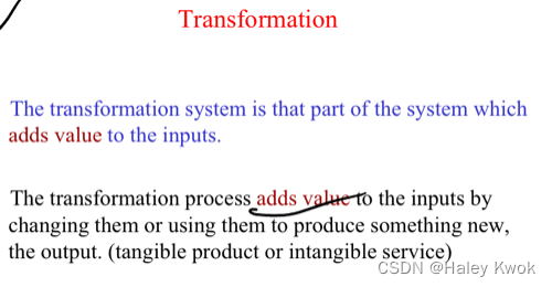
Transformation
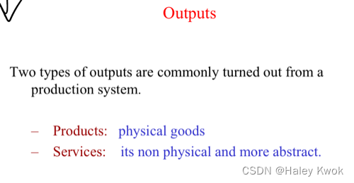
Outputs
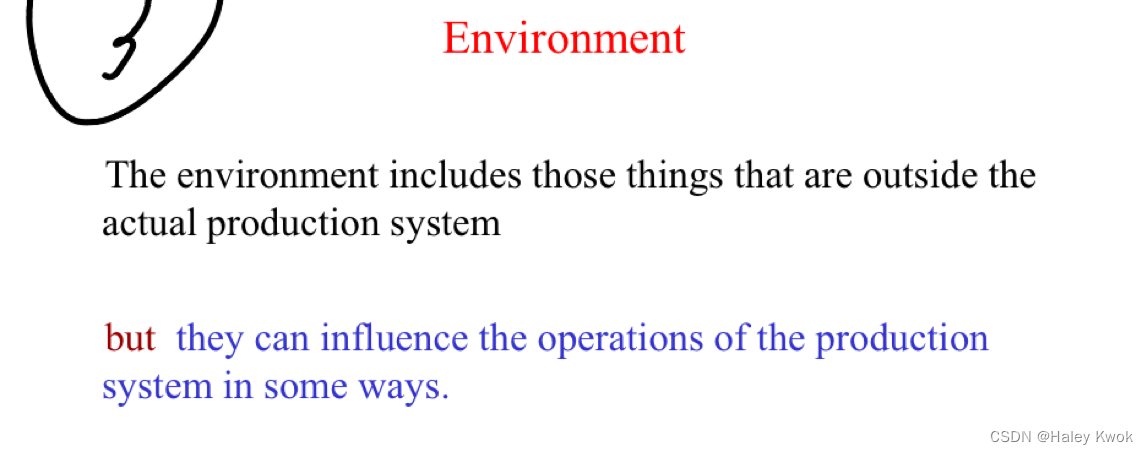
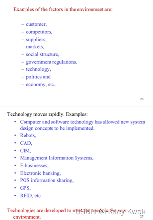
Environment
Example

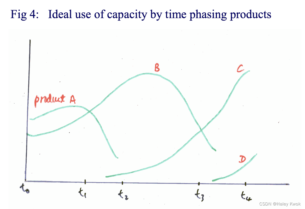
Chapter 2: Capacity Planning
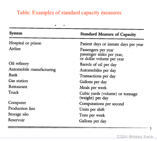
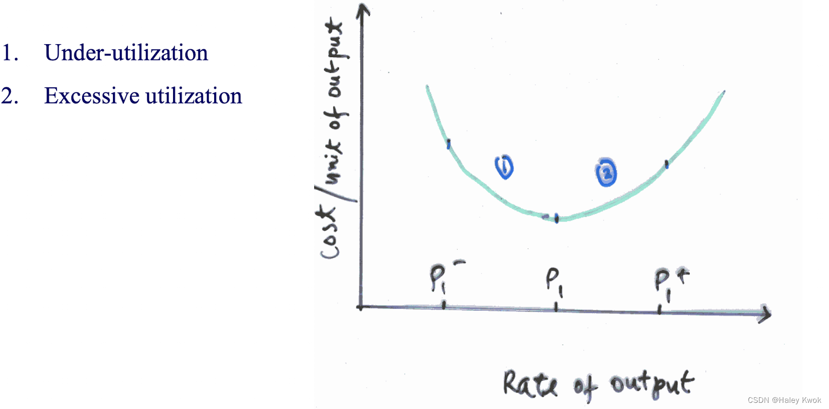
Capacity of a facility: the maximum rate of production or service capability of a company’s operation.
Usually expressed as L volume of output per time period. (e.g., units/week, customers/hr et.)
1. Design Capacity
The maximum output that can possibly be attained per unit time.
2. Effective Capacity
The maximum possible output attainable per unit time given
– a product mix,
– scheduling difficulties,
– m/c maintenance,
– quality factor, etc
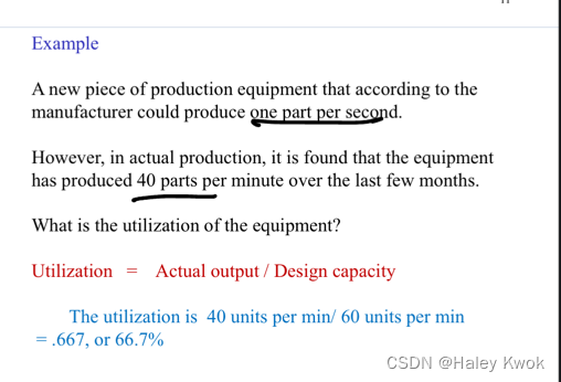
Actual output: The output per unit time actually achieved.
Efficiency = Actual output / Effective capacity
Utilization = Actual output / Design capacity
Example
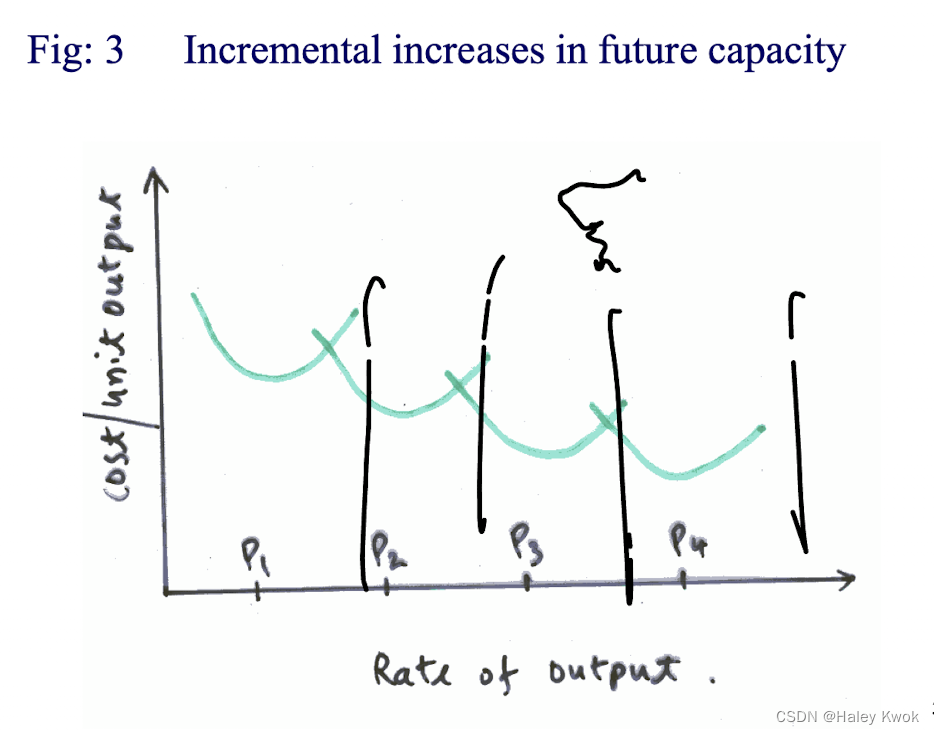
3. Strategies for Modifying Capacity

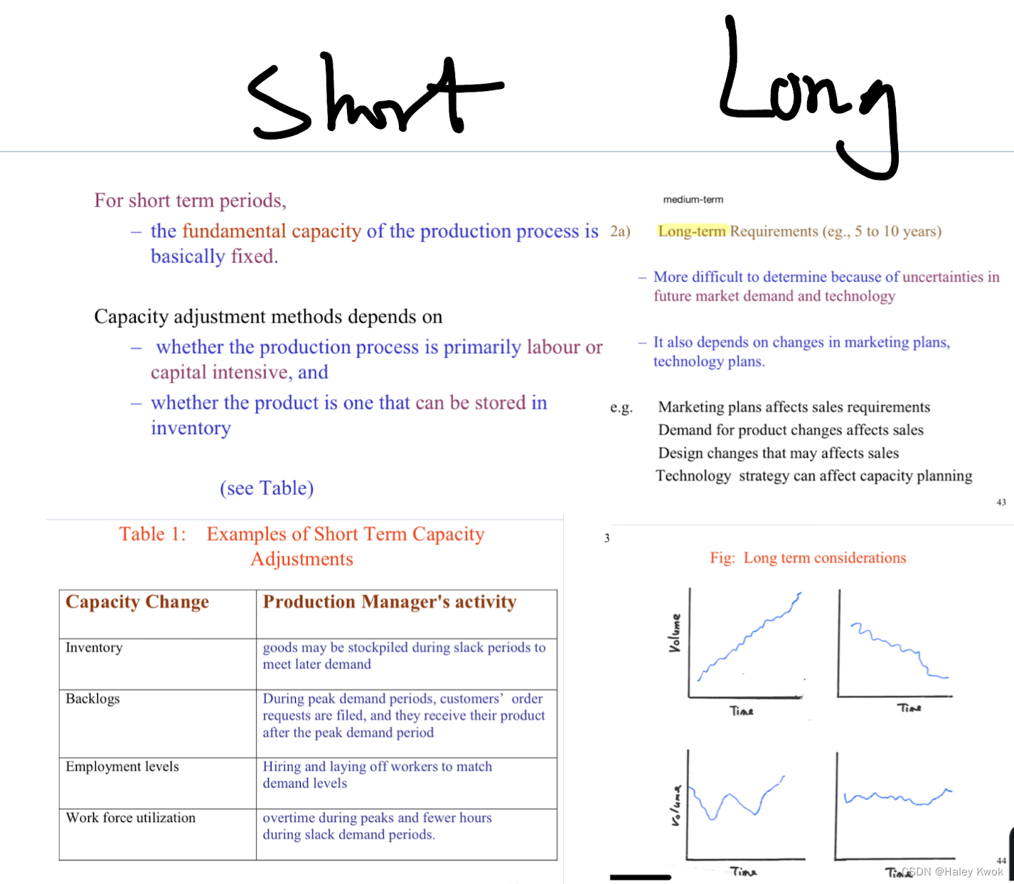
Product = Sale Revenue - Cost (fixed + variable)

Expansion
If demand is anticipated to be permanently higher, facilities should be expanded to heap the benefits of economics of scale offered by a larger facility.
Contraction and Constant Capacity
Selling off existing facilities, equipment and inventory; firing employees (last resort).
Seeking new ways to maintain and use existing capacity.
Chapter 3: Forecasting
Demand Forecast:
– The estimation of the future trend and expectation of
the demand of a business based on analysis of past data, or on judgement and opinion
e.g., long range/ medium range/ short range demand forecast
Elements of a Good Forecast
Timely: the forecasting horizon must cover the time necessary to implement possible changes.
Accurate: the degree of accuracy (possible error) should be stated. Reliable: a forecast technique should work consistently.
Simple and easy: forecasts should be made in simple and written forms that can be easily understood and used.
Cost effective: the benefit should outweigh the costs.
External
Available statistics: e.g.
– The national Economic Health Pricing Index,
– Consumers - spending trends,
– Trading, import and export figures, etc
Internal
Data specific to the products of the company, eg:
- Historical Data (sales records, customer orders, production orders….)
- Opinions:
Consumer Opinion, Customer Opinion, Executive Opinion - Market Research
- Marketing Trials
- Distributor Survey
Approaches to Forecasting
Forecasting Procedure:
The basis steps are:
- Identify the product or service (group) for demand forecast.
- Determine the purpose of the forecast.
- Establish a time horizon.
- Select a forecasting technique.
- Collect, clean and analyze appropriate data.
- Make the forecast.
- Monitor the forecast.
Qualitative: Forecast based on subjective inputs. (Delphi Method, Expert judgement, executive opinions, sales force opinions, consumer surveys.)
Quantitative: Forecast based on analysis of historical data or causal variables. (Time series models, trend projection methods, regression analysis)
Qualitative Forecasting Techniques
- Consumer Survey: The opinions of consumers are surveyed and analysed to
produce the forecast. - Sales Force Composite Method: Opinions of sales and marketing people are taken and analysed to produce the forecast.
- Jury of Executives Opinion: Opinions of executives are taken and analysed to produce the forecast.
The Delphi Technique:
- In this method, a attempt is made to develop forecasts through “group consensus” by the knowledgeable people/experts.
- Series of questionnaires are answered anonymously by members of the panel.
- The goal is to produce a relatively narrow spread of opinions within which the majority of the members concur.
- Generally used for long range forecasts. (Others, eg., regarding scientific advances, changes in society, government regulations, and the competitive environment, etc )
Quantitative Forecasting Techniques (Forecasting Models):
Broadly speaking,
– 2 basic types of techniques:
1) Time Series Model
Here, the variables to be forecasted is analysed historically over time and the pattern or patterns are modelled and estimated.
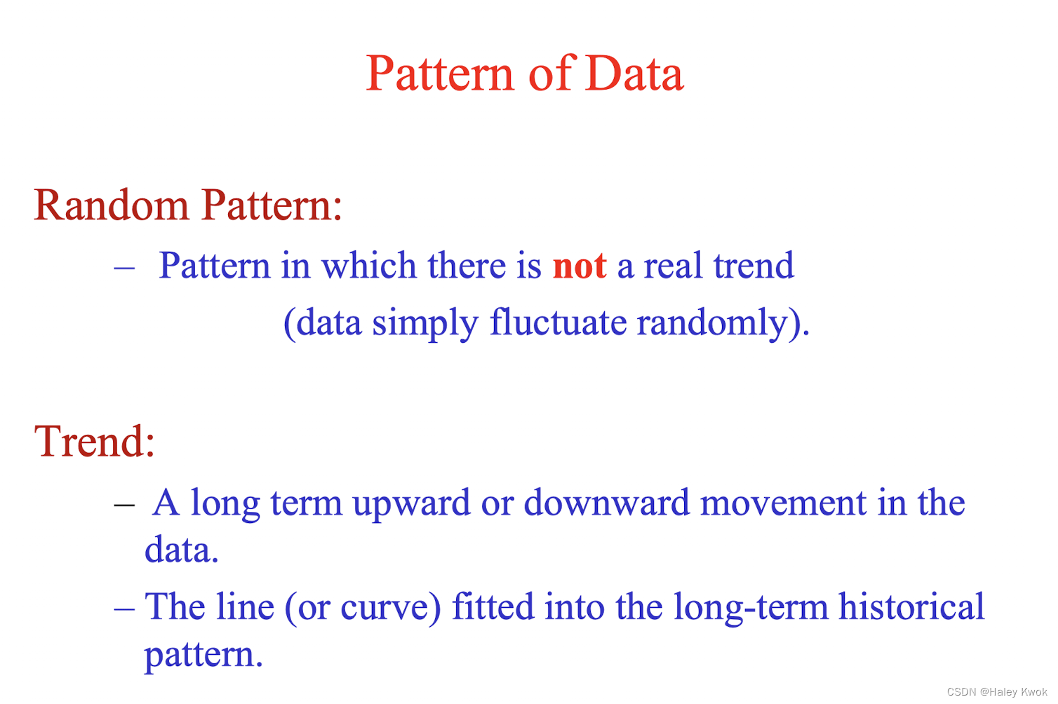
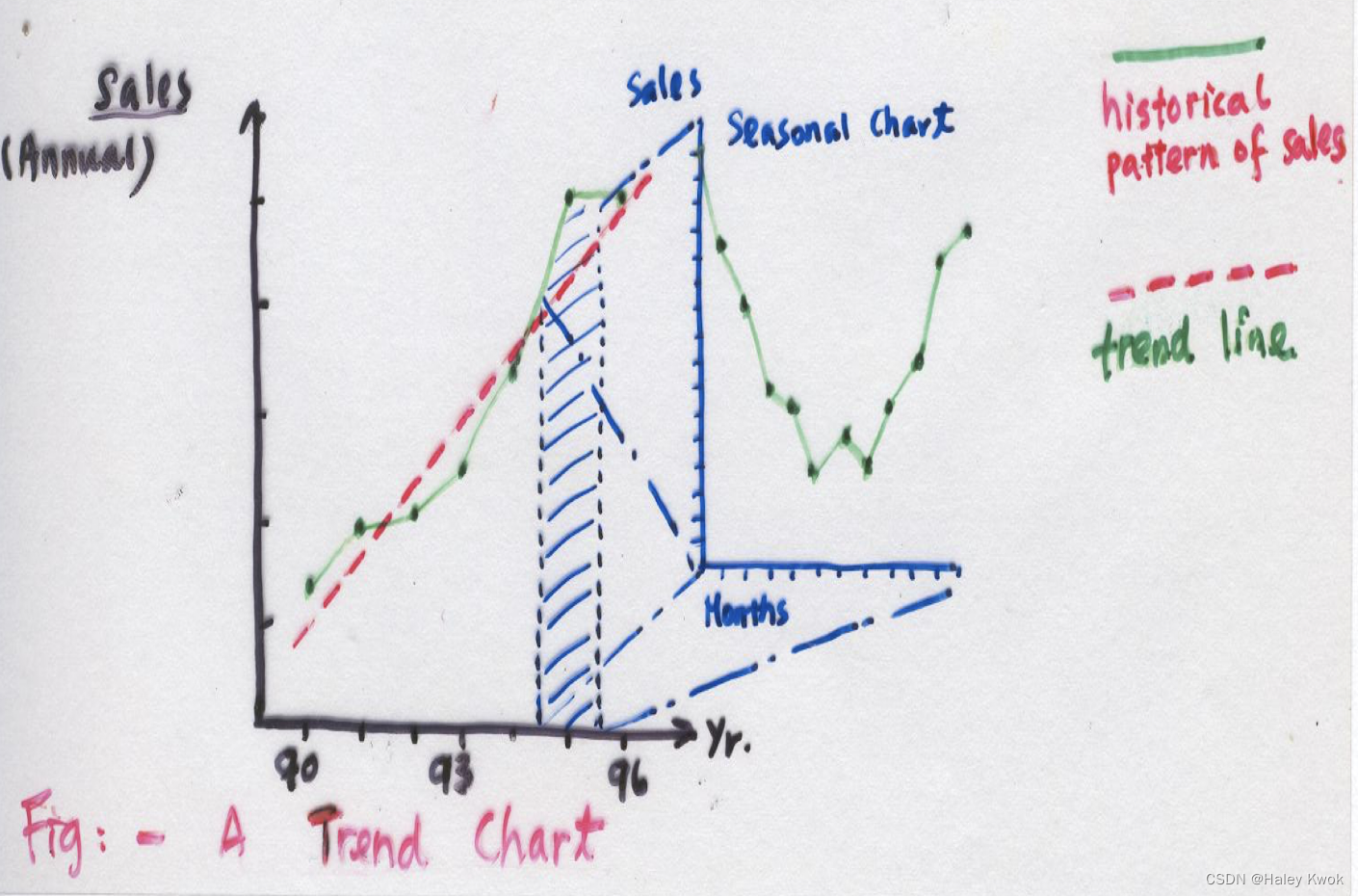
Seasonal Fluctuation (Seasonality)
Pattern in which fluctuations in the data
– occur during some fixed time period of one year or less according to some seasonal factor,
– repeats itself over each consecutive time period.
Cyclical Variation
Pattern which is similar to the seasonal pattern, except that
– the time period is not one year and
– the cycles do not necessarily form a repeating pattern.
– the magnitude, timing and pattern of cyclic fluctuation vary so widely and are due to so many causes.
– generally impractical to forecast them.
Irregular variations
– Variations due to unusual circumstances.
– Their inclusion can distort the overall picture and should be identified and removed from the data.
Residual Unexplained Variations
– The elements which can not be forecasted.
e.g. “Acts of God”, sudden change in politics.

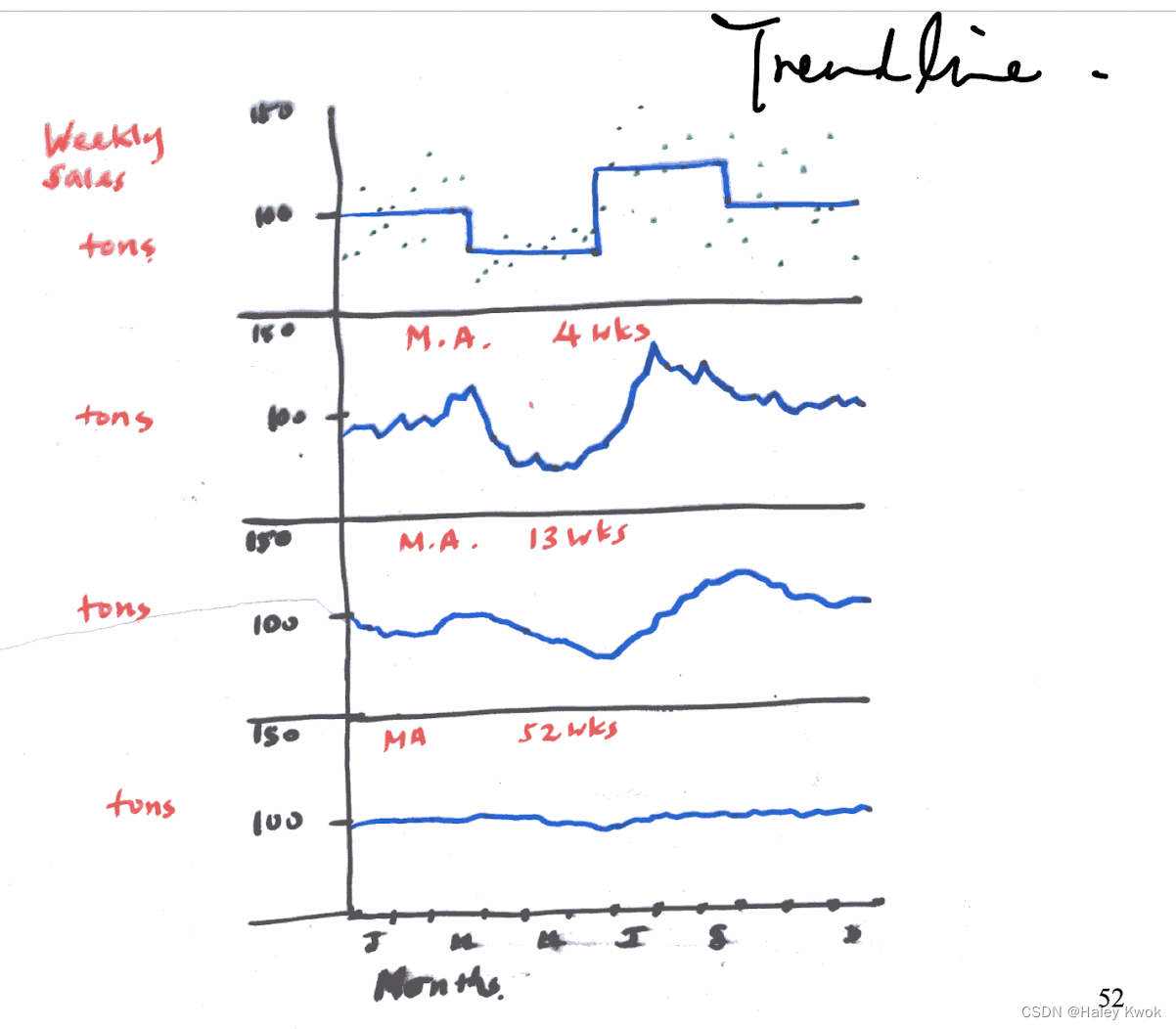
1) Moving Average:
A moving average forecast is obtained by summing and averaging the data points over a desired number of past periods (N).
– This number usually encompasses a seasonal cycle in order to smooth out seasonal variations.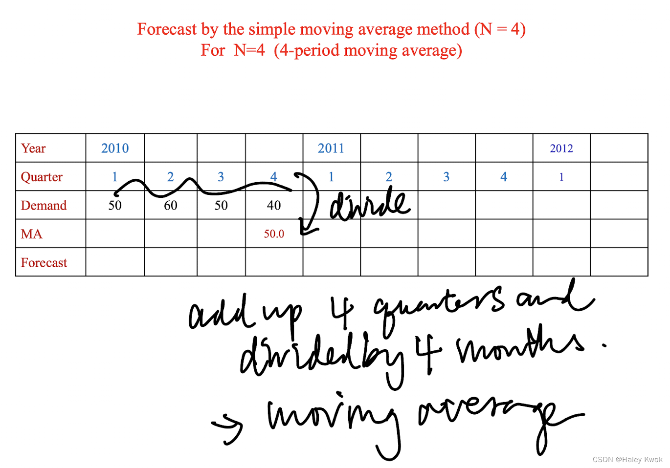
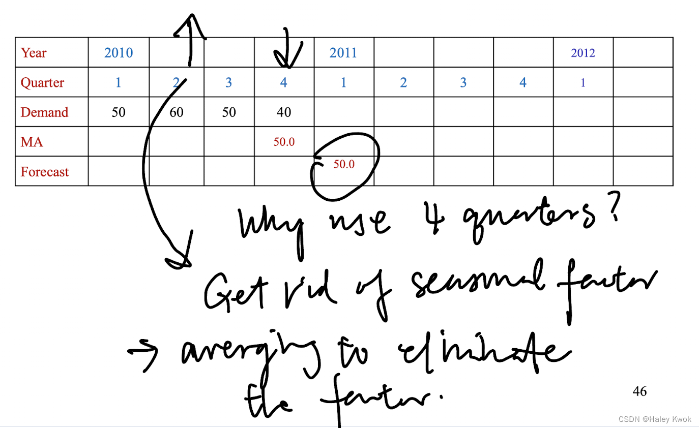
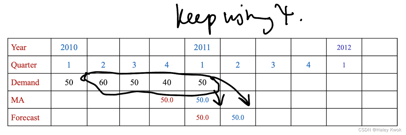
Characteristics
– The method is not influenced by very old data
– The method does not reflect solely the figure for the previous period.
– It smoothes the pattern of figures.
– It indicates the trend of the figures
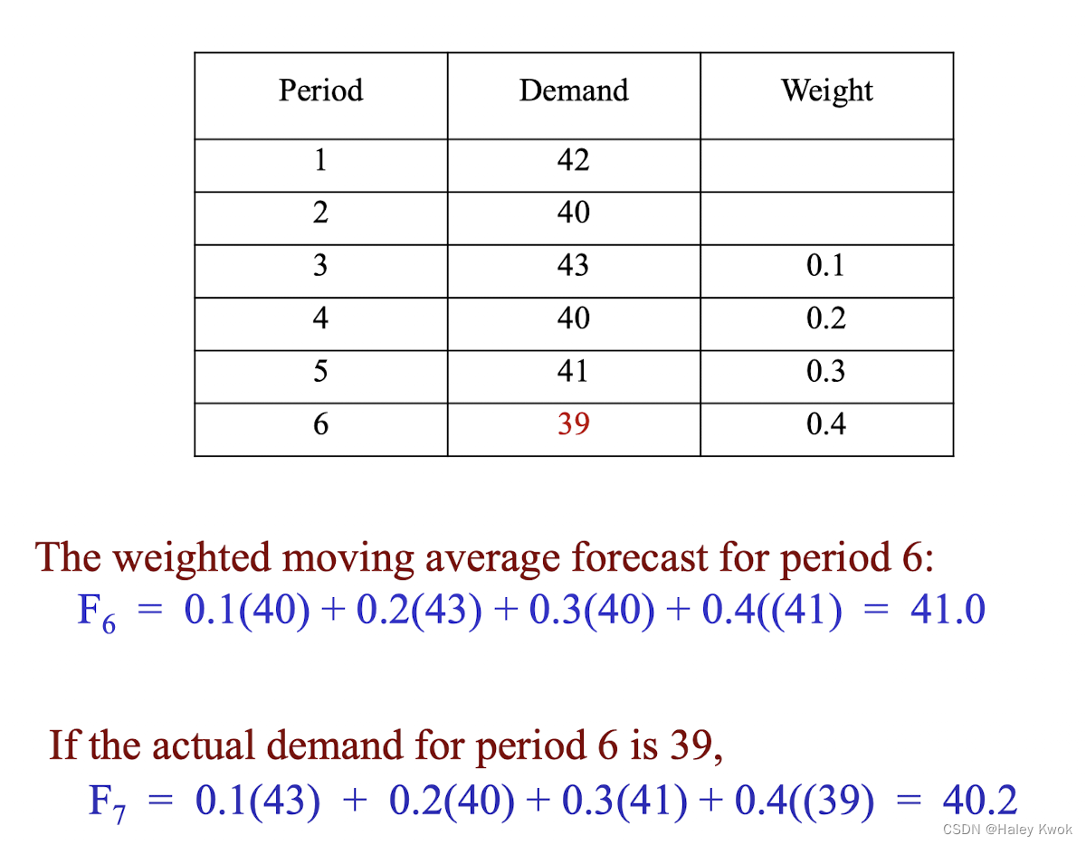
2) Weighted moving average
It is similar to moving average
– Except that it is more reflective of the recent occurrences, (usually it assigns more weight to the most recent values in a time series.)
– The weights must sum to 1.00.

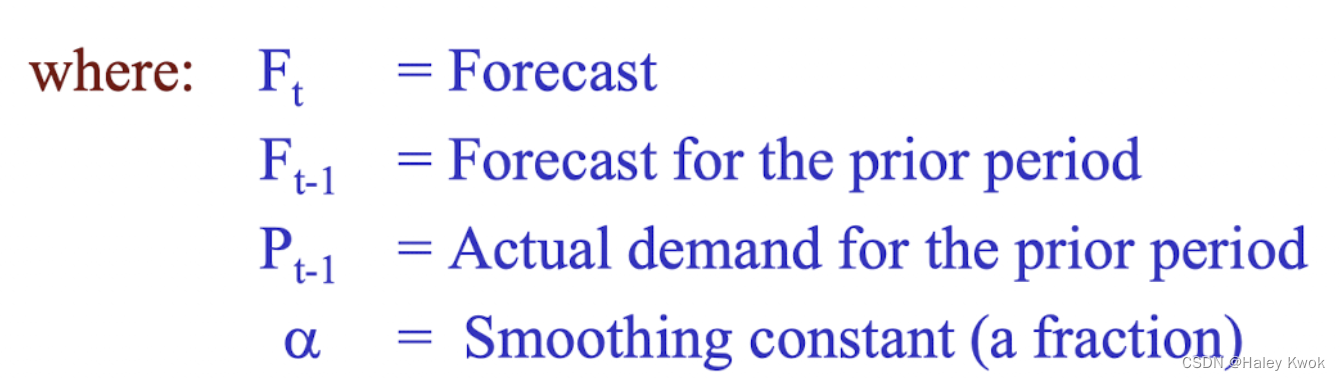
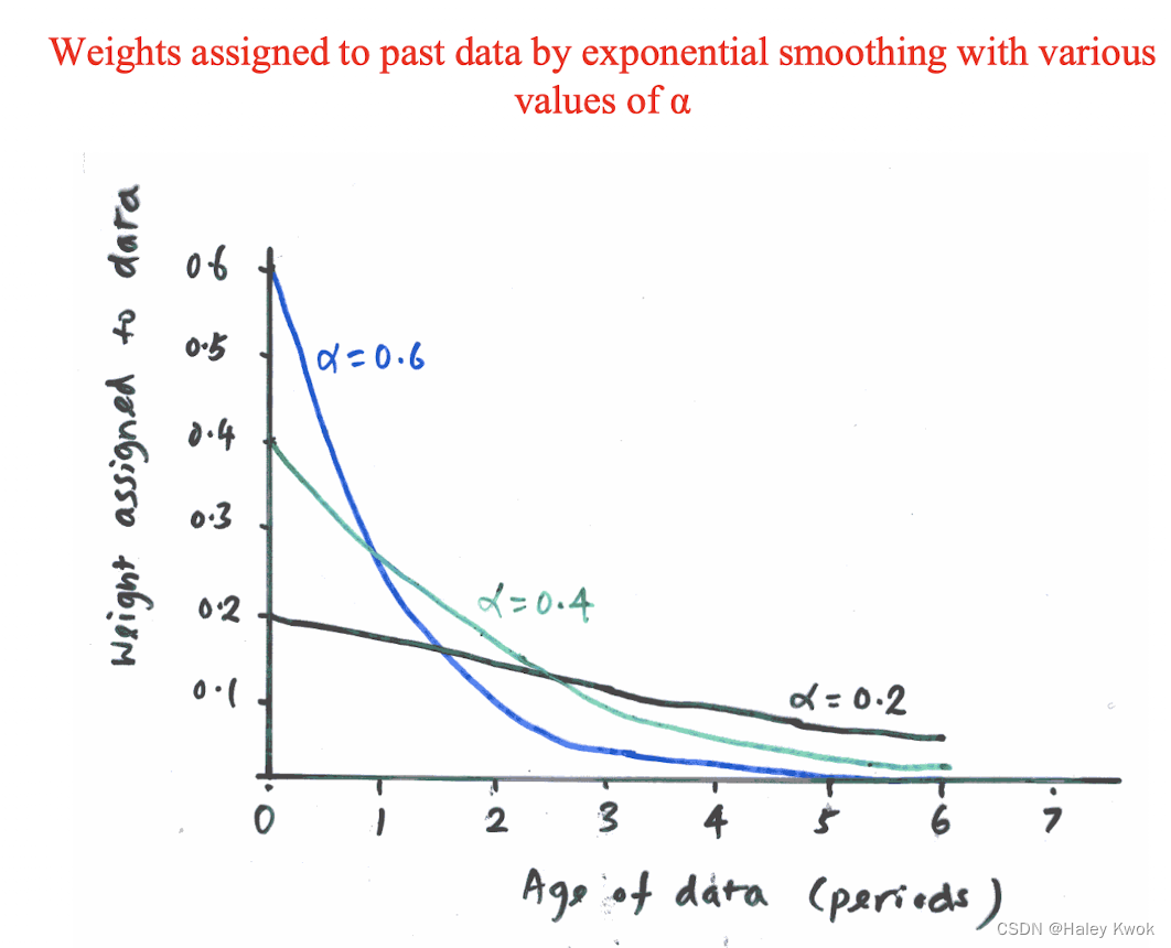
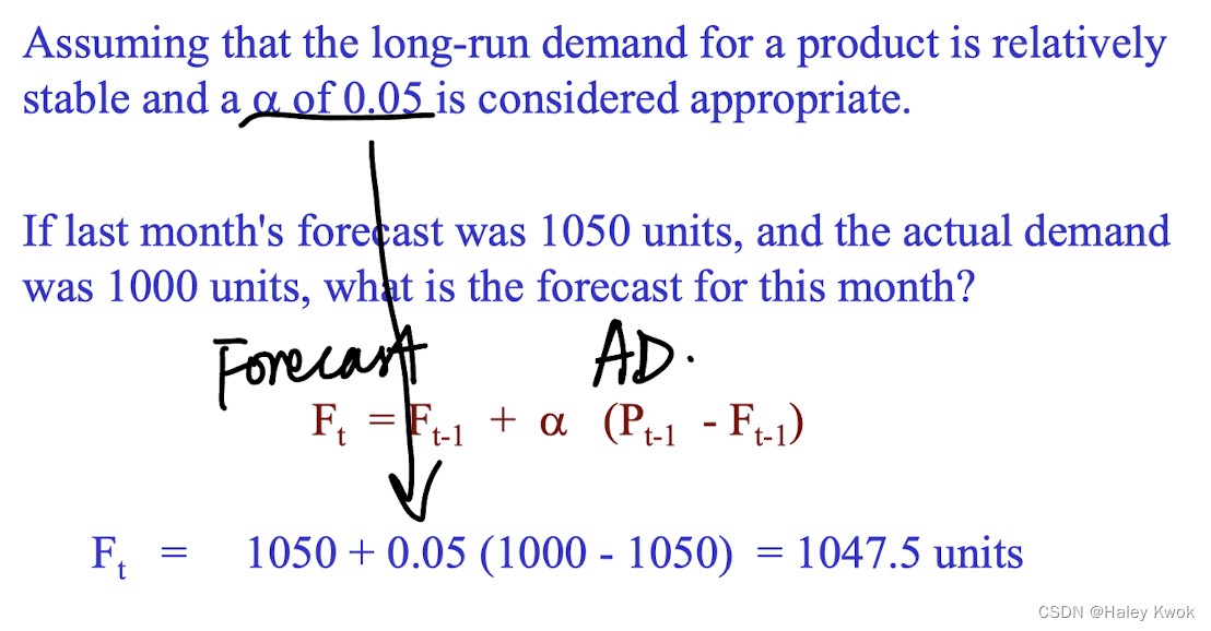
3) Exponential Smoothing
A weighted average method based on the previous forecast plus a fraction/percentage (alpha) of the difference between that forecast and the actual demand of the period.
ie: The forecast for any period = The forecast for the prior period + A fraction of the error in the forecast for the prior period.
Equation used for forecasting:
F t = F t − 1 + α ( P t − 1 − F t − 1 ) F_t = F_{t-1} + \alpha (P_{t-1} - F_{t-1}) Ft=Ft−1+α(Pt−1−Ft−1)
An equivalent formula:
F t = α P t − 1 + ( 1 − α ) F t − 1 F_t = \alpha P_{t-1} + (1-\alpha) F_{t-1} Ft=αPt−1+(1−α)Ft−1
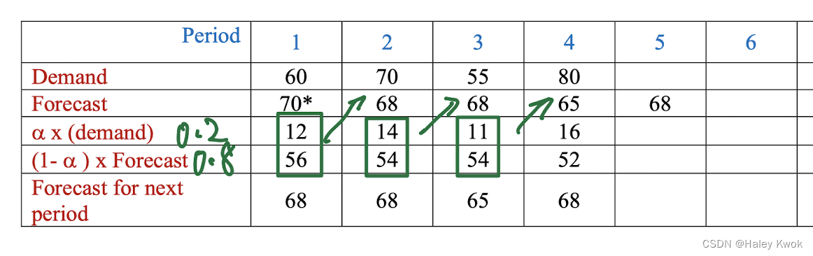
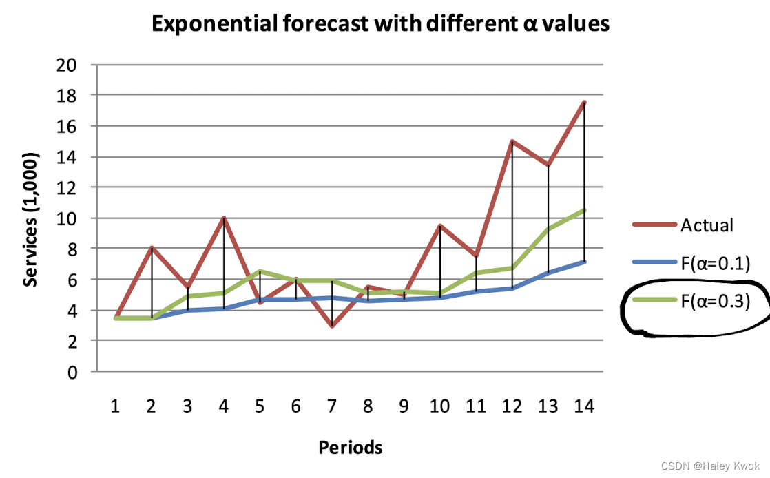
Interpretation: the demand during 1 and 2 increases, while the forecast for next period remain the same, showing that the chosen alpha value is not sensitive enough to the changes.
Choice of alpha value
alpha can be between >0 to <1.
Higher the alpha value, greater the weight given to the recent demands.
Commonly used values range from 0.1 to 0.5
Mean Absolute Deviation (MAD)
Error = Actual - Forecast
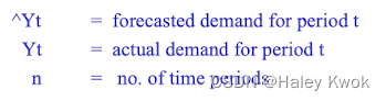
M A D = ( ∑ ∣ Y t − Y t ∣ ) / n MAD = ({\sum} |Y_t - ^ Yt| ) /n MAD=(∑∣Yt−Yt∣)/n
Bias
A measure of the tendency to consistently over or under forecast (error). It is an indication of the directional tendency of forecast errors.
M A D = ( ∑ Y t − Y t ) / n MAD = ({\sum} Y_t - ^ Yt) /n MAD=(∑Yt−Yt)/n
The value of alpha = 0.3 is chosen because of the smaller MAD and Bias resulted.
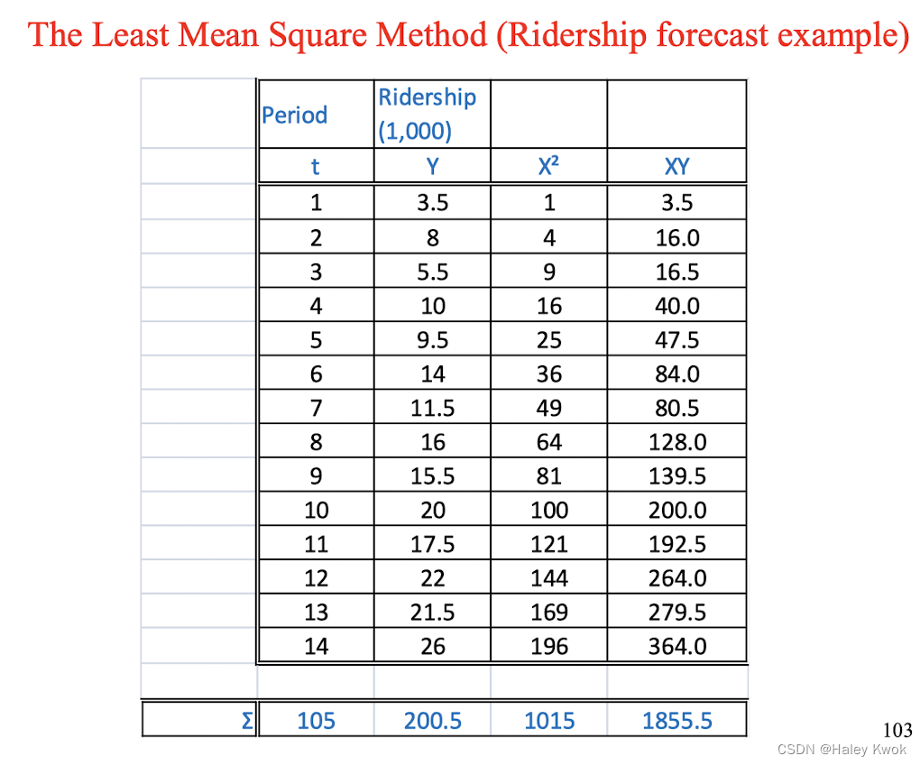
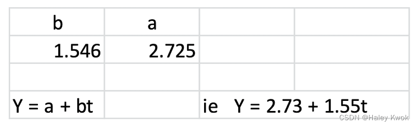
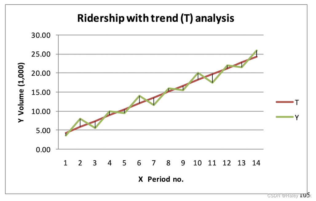
**Least Mean Squares Method
It is a method for trend analysis which involves developing an equation that will suitably describe a linear trend.
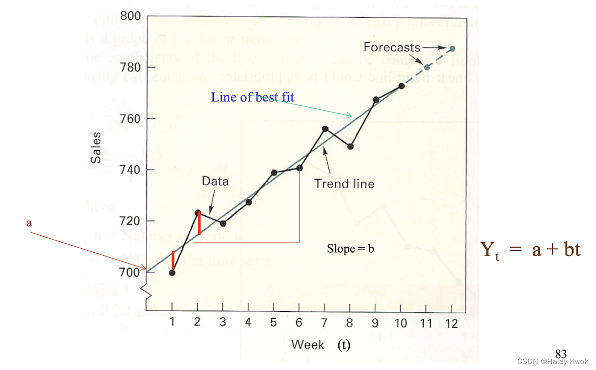
Y t = a + b t Y_t = a + bt Yt=a+bt
To determine a and b:
N = No. of data
∑ Y = N a + b ∑ t {\sum}Y = Na + b {\sum}t ∑Y=Na+b∑t
∑ t Y = a ∑ t + b ∑ t 2 {\sum}tY = a {\sum}t + b {\sum}t^2 ∑tY=a∑t+b∑t2
Examples: 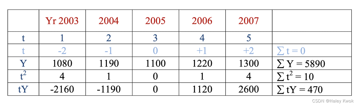
∑ Y = N a + b ∑ t {\sum}Y = Na + b {\sum}t ∑Y=Na+b∑t
5890 = 5a + b (0)
a = 1178
∑ t Y = a ∑ t + b ∑ t 2 {\sum}tY = a {\sum}t + b {\sum}t^2 ∑tY=a∑t+b∑t2
470 = 0 + 10b
b = 47a = 1178 x 1000 = 1178000
b = 47 x 1000 = 47000
Yt = 1178000 + 47000tForecast for the year 2008 (t = 3):
Yt = 1178000 + 47000t
= 1178000 + 47000 x 3
1319000//
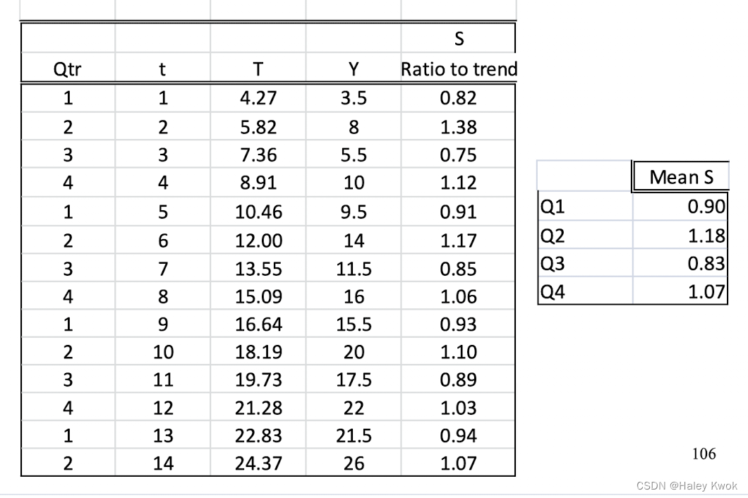
Determination of the Seasonal Component
Multiplicative Seasonal Method
It adjusts a given forecast by multiplying the forecast by a seasonality factor.
Seasonal Factor: The index of the “average” periodic demand that occurs in each period.
Example: The “Quarterly Average Method”
Quarterly Seasonality Factor = Quarterly demand / Quarterly average
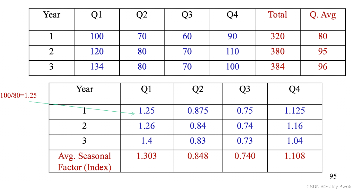
Example: The “Ratio to Trend Method”
Adjusted the forecast by seasonal factors
We can compute, say, for each available quarter of data, a measure of the “seasonality” in that quarter by
S = Y i / Y i S = Yi/ ^Yi S=Yi/Yi

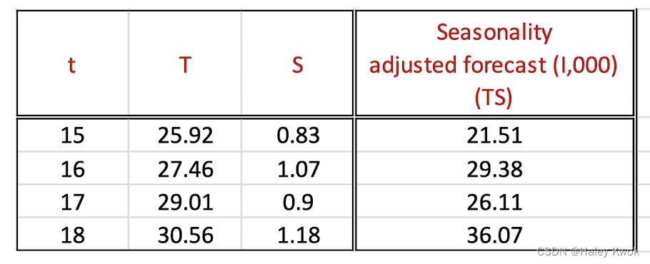
Determination of mean seasonality index
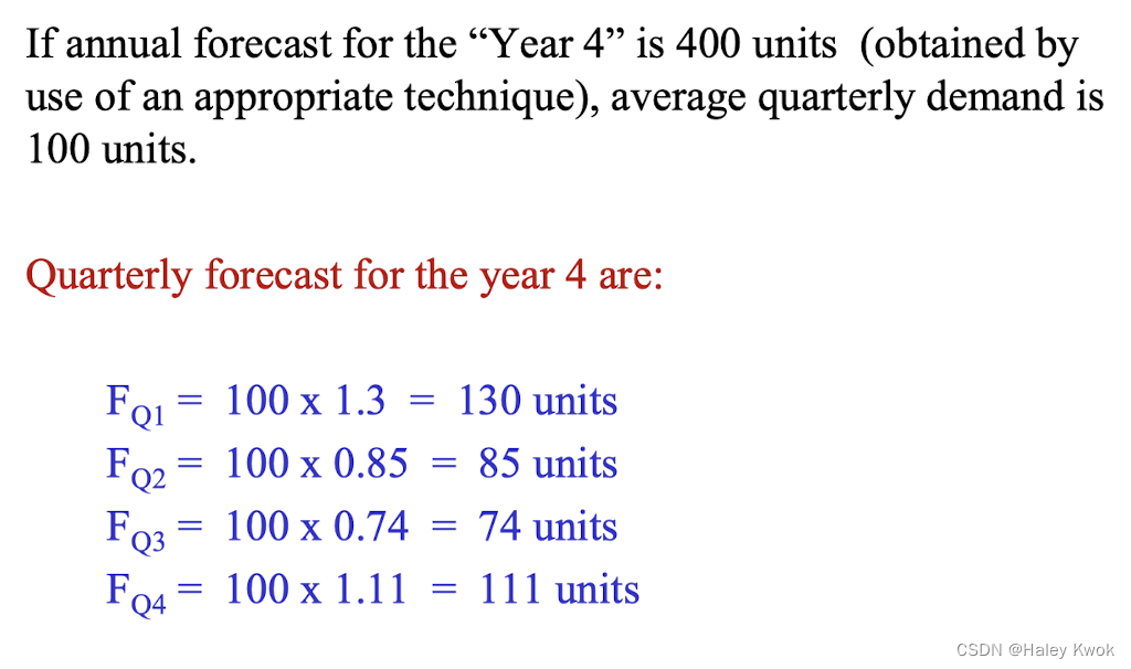
Seasonality adjusted forecast for periods 15 to 18 are
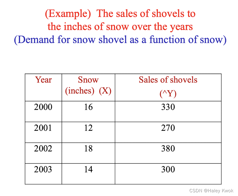
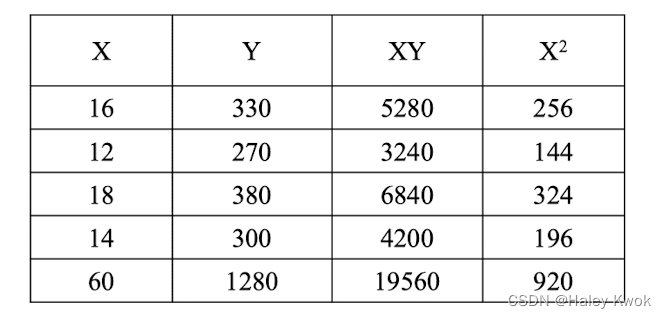
2) Causal Model
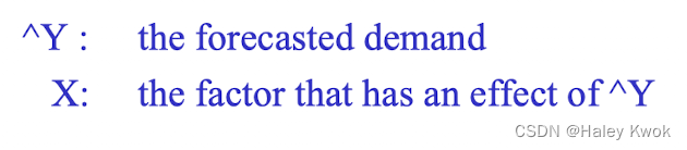
Here, the variables which are related to the entity to be predicted are delineated, and their predictive relationship to it is modelled and used for forecasting.
Here, the factors (independent variable) that cause the demand (dependent variable) are being identified and used to forecast the demand.
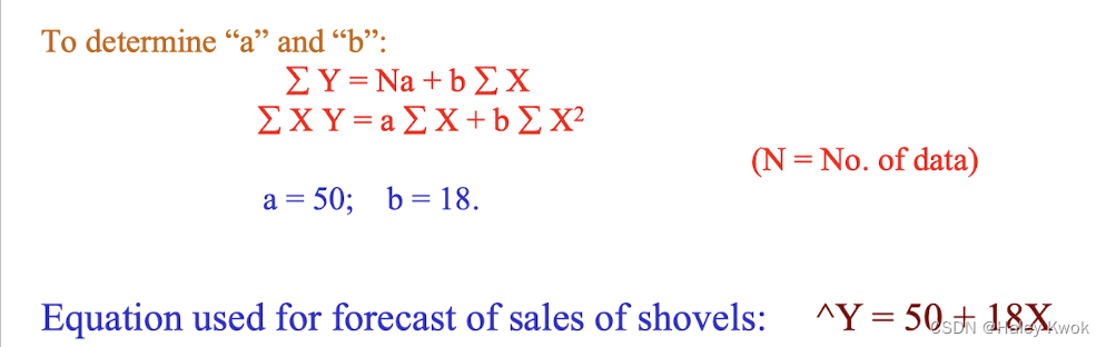
Simple Linear Regression
The least mean square method used in the preceding section
can also be used to estimate a predicting equation for a
demand in future:
Y = a + b ^Y = a + b Y=a+b
Multiple Linear Regression
The linear regression methodology can be extended to
situations where more than one variable is used to explain
the behaviour of the dependent variable Y.
3) Econometric models
The dependent and independent variables used in forecasting models are interdependent. (e.g., the demand may be a function of personal income and personal income a function of demand, etc…)
Forecast Accuracy and Control
Accuracy: the extent to which the forecast deviates from the actual value
Error = Actual - Forecast
M A D = ( ∑ ∣ Y t − Y t ∣ ) / n MAD = ({\sum} |Y_t - ^ Yt| ) /n MAD=(∑∣Yt−Yt∣)/n
M A D = ( ∑ Y t − Y t ) / n MAD = ({\sum} Y_t - ^ Yt) /n MAD=(∑Yt−Yt)/n
- Mean square error (MSE)
[ ∑ ( Y t − Y t ) 2 ] / ( n − 1 ) [{\sum} (Yt - ^Yt)^2] / (n-1) [∑(Yt−
 最低0.47元/天 解锁文章


 327
327

 被折叠的 条评论
为什么被折叠?
被折叠的 条评论
为什么被折叠?
 到【灌水乐园】发言


