2024.6.23周报_nas-pinn代码-CSDN博客

本文链接：https://blog.csdn.net/m0_68477761/article/details/139862787

摘要

ABSTRACT

摘要

本周阅读了一篇题目为NAS-PINN: NEURAL ARCHITECTURE SEARCH-GUIDED PHYSICS-INFORMED NEURAL NETWORK FOR SOLVING PDES的文献，文章提出了一种神经结构搜索引导方法，即NAS-PINN，用于自动搜索求解特定偏微分方程的最优神经结构。其次通过代码实验，对一个偏微分方程进行求解，加深了自己对求解步骤的理解。

ABSTRACT

This week, I read a paper titled "NAS-PINN: Neural Architecture Search-Guided Physics-Informed Neural Network for Solving PDEs." The paper proposes a neural architecture search-guided method, NAS-PINN, to automatically search for the optimal neural architecture for solving specific partial differential equations (PDEs). Additionally, by conducting a code experiment to solve a PDE, I gained a deeper understanding of the solving steps.

一、文献阅读

一、题目

1、题目：NAS-PINN: NEURAL ARCHITECTURE SEARCH-GUIDED PHYSICS-INFORMED NEURAL NETWORK FOR SOLVING PDES

2、期刊：Journal of Computational Physics

3、链接：https://arxiv.org/pdf/2305.10127

二、摘要

通过损失函数将物理信息纳入神经网络，可以以无监督的方式预测偏微分方程的解，然而，神经网络结构的设计基本上依赖于先验知识和经验，因此，本文提出了一种神经结构搜索引导方法，即NAS-PINN，用于自动搜索求解特定偏微分方程的最优神经结构。文章通过将搜索空间松弛为连续空间，并利用掩模实现不同形状张量的添加，NAS-PINN可以通过双级优化进行训练，其中内环优化神经网络的权重和偏置，外环优化结构参数。同时，研究发现，更多的隐藏层并不一定意味着性能更好，对于泊松和平流方程，一个神经元较多的浅神经网络在pinn中更合适。

By incorporating physical information into the neural network through the loss function, it can predict solutions to partial differential equations (PDEs) in an unsupervised manner. However, the design of the neural network structure largely relies on prior knowledge and experience. Therefore, this paper proposes a neural architecture search-guided method, namely NAS-PINN, to automatically search for the optimal neural architecture for solving specific PDEs. By relaxing the search space into a continuous one and utilizing masks to realize the addition of tensors in different shapes, NAS-PINN can be trained through a bi-level optimization, where the inner loop optimizes the weights and biases of the neural network, and the outer loop optimizes the architecture parameters. It is also found that more hidden layers do not necessarily mean better performance. For Poisson and Advection equations, a shallow neural network with more neurons is more suitable in PINNs.

三、网络架构

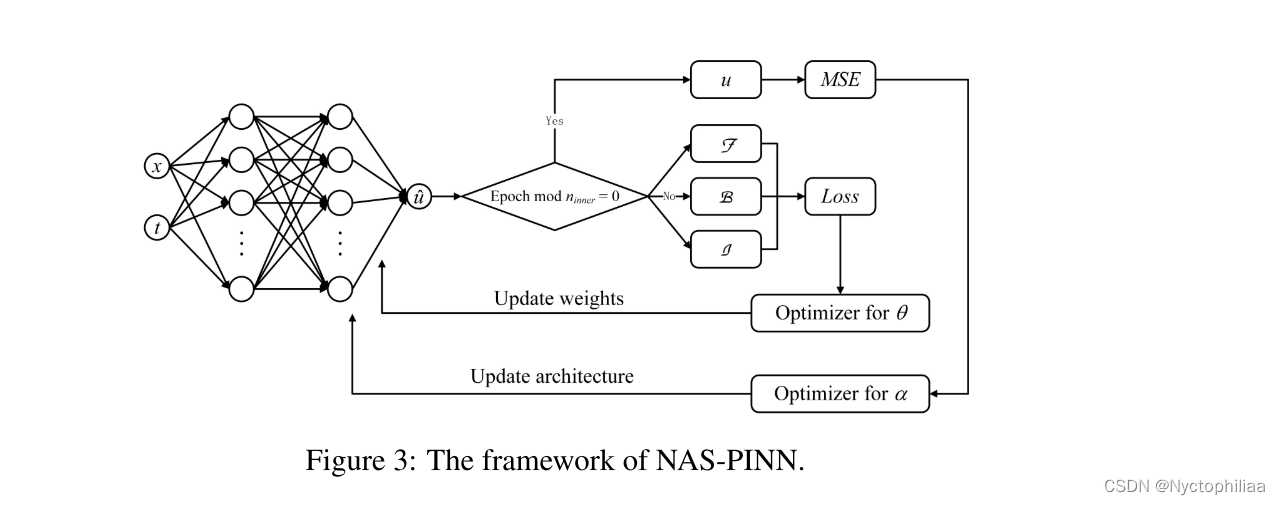
四、创新点

1、提出了一种基于搜索引导的物理信息神经网络(NAS-PINN)的神经网络结构。

2、实现了在有限的数据量下自动搜索求解给定PDE的最佳神经结构。

3、掩模用于张量相加，以帮助搜索每层中不同数量的神经元。

五、文章解读

1、Introduction

本文探讨了使用物理信息神经网络来求解偏微分方程。传统的数值方法，如有限差分法、有限元法和有限体积法，尽管在精度上表现优异，但随着维度的增加，其计算成本也呈指数增长，导致维度灾难。解决PDE的深度学习方法主要有两类：学习神经算子和使用PDE作为约束。前者需要大量的数值结果作为训练数据，训练完成后，可以处理具有相同形式但不同参数的PDE。然而，这种方法完全依赖数据驱动，忽略了PDE的物理信息。PINN通过定义适当的损失函数将物理信息嵌入神经网络中，利用自动微分技术简化偏导数计算，已被证明在求解PDE和发现PDE参数方面有效。在原始的PINN框架中，边界条件和初始条件通过定义的损失函数软约束。为了保证约束，简单形式的边界和初始条件可以显式编码到神经网络中。目前，PINN中的神经网络设计主要依赖于先验知识和经验，通常采用4到6个隐藏层且每层有相同数量的神经元。为解决这一问题，本文提出了一种神经架构搜索引导方法，即NAS-PINN，通过结合NAS方法自动搜索最佳神经网络架构来求解特定PDE。

2、Method

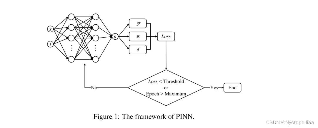
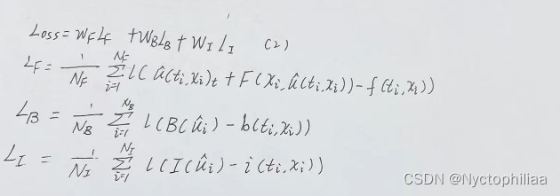
1、PINN

2、Differentiable NAS

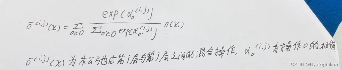
在传统的NAS算法中，神经网络的层数通常是固定的，并为每一层提供特定的操作选择。这种配置使得搜索空间不连续，无法通过基于梯度的方法进行优化，极大地限制了算法的收敛速度和效率。

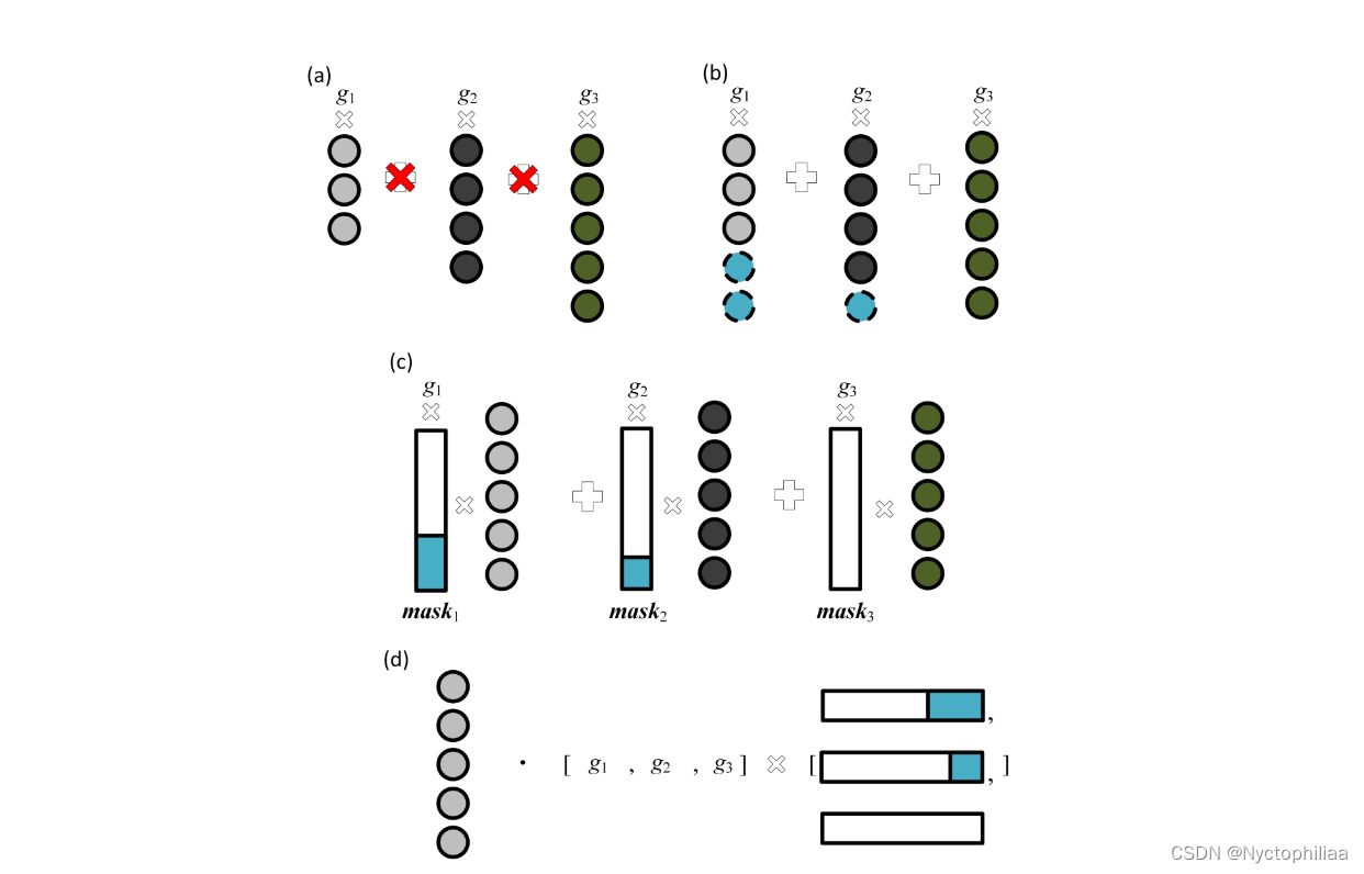
3、Masks

虽然Differentiable NAS将搜索空间简化为连续空间，但张量操作只允许添加相同形状的张量，使得搜索神经元数量变得不切实际，如下图(a)所示。受卷积神经网络中填充零的启发，我们可以将神经元填充到最大数量k，如下图(b)所示。在下图(c)中，通过将填充的神经元乘以1 - 0张量掩模，停用了额外的神经元以模拟不同数量的神经元。

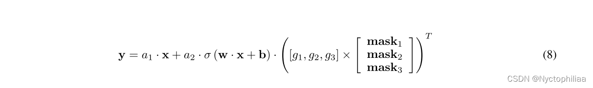
最后通过权值共享，可以将可选的隐藏层减少到1个，输出y可以表示为:

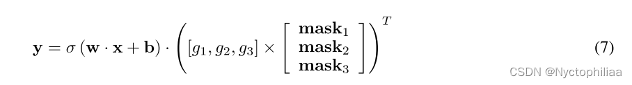
其中σ(·)为激活函数，w和b为单个隐藏层的权重和偏置， $g_{i}$ 为每个神经元数量的权重标量， $mask_{i}$ 为每个神经元数量的掩模，其形状为1 × k。则mask的前第j个元素为1，其余(k−j)个元素为0。

为了确定层数，引入恒等变换作为操作，表示跳过这一层，输出y变为

根据权值a选择最合适的层，通过权值g决定每层中最合适的神经元。这里我们将a和g统称为 $\alpha$ ， w和b统称为 $\theta$ 。

3、实验

考虑一系列偏微分方程来测试所提出的NAS-PINN，并试图找出解决偏微分方程的有效神经结构的特征。文章中考虑了泊松方程、Burgers方程和平流方程。

1、泊松方程

神经元数量与隐藏层数量如下表所示：

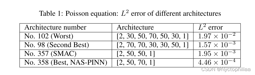
序列的第一个和最后一个元素表示输入和输出通道，而其他元素表示每层的神经元数。例如，体系结构No.98的输入大小为n × 2，其中n为批大小，2代表坐标x和y，第一个隐藏层有70个神经元。

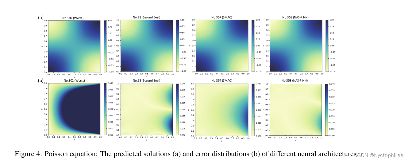
从表1和图4中我们可以清楚地看到，NAS-PINN神经结构的 $L^{2}$ 误差最小，其误差分布也比其他结构有所改善。因此，所提出的NAS-PINN确实在给定的搜索空间中找到了最佳的神经结构。虽然98号架构也表现出了相对较好的性能，但它的参数比NAS-PINN架构要多得多。这表明更多的参数并不一定意味着更好的性能。

2、Burgers方程

这里考虑具有周期边界条件的时变一维Burgers方程:

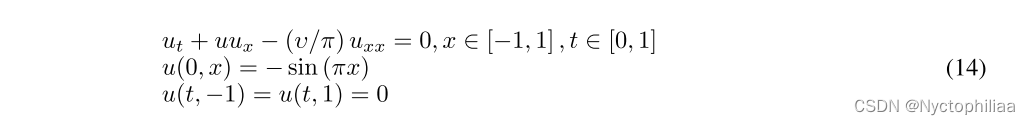
研究了具有不同υ值的Burgers方程，并通过Chebyshev谱法得到了参考解。在架构搜索阶段，我们均匀地沿t轴取21个点，沿x轴取250个点。同样的点被用来从头开始训练所有的神经结构。沿t轴均匀采样21个点，沿x轴均匀采样500个点，检验所有的收敛模型。表3和图8和图9给出了不同扩散系数υ的Burgers方程的结果。实验重复5次，计算平均值。

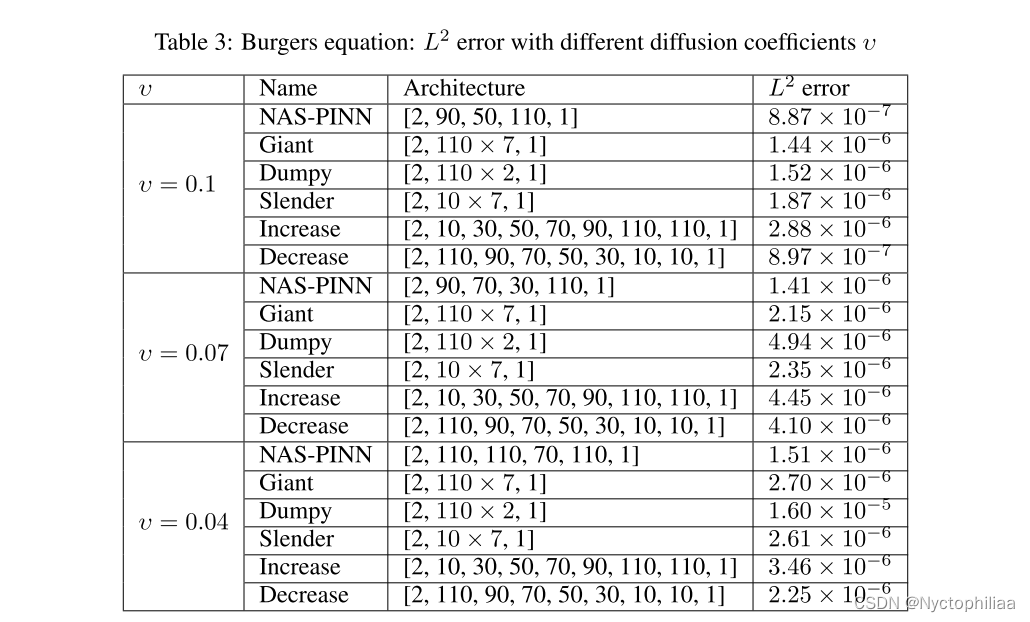
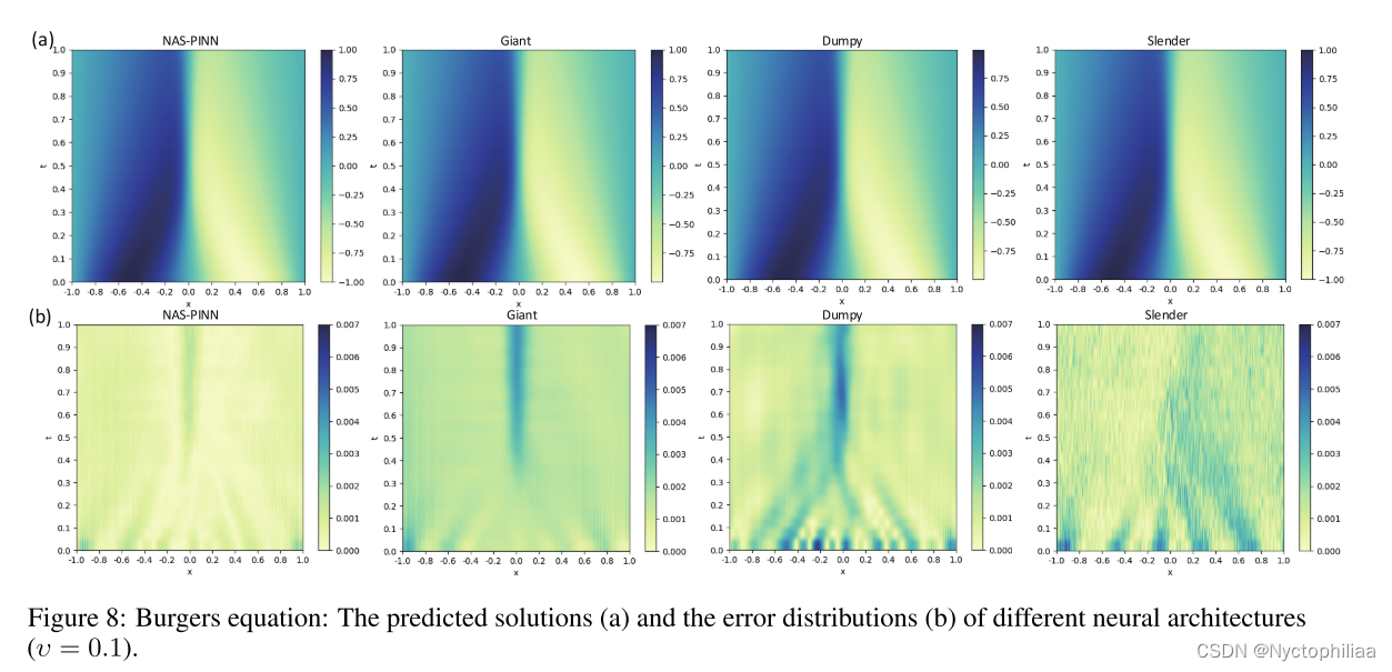
研究发现，NAS-PINN搜索架构的预测比参考架构的预测更准确，当υ = 0.1时这种优势尤为明显。NAS-PINN搜索的架构通常有3或4个隐藏层，这比最大数量要小得多，进一步证明了更深的神经网络不一定能产生更好的结果，对于某个问题确实存在最佳的隐藏层数。

3、平流方程

这里，我们考虑一个一维平流方程:

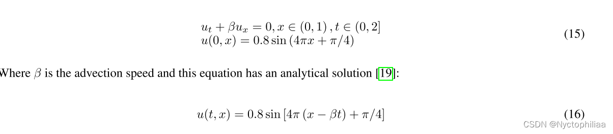
研究了不同β值下的平流方程。搜索空间和参考神经结构与上述相同。沿t轴均匀取40点，沿x轴均匀取120点作为建筑搜索阶段。同样的点被用来从头开始训练所有的神经结构。沿t轴均匀采样40个点，沿x轴均匀采样120个点，检验所有训练好的模型。表4和图10、图11给出了不同平流速度β下平流方程的结果，平均值取自5次独立实验。

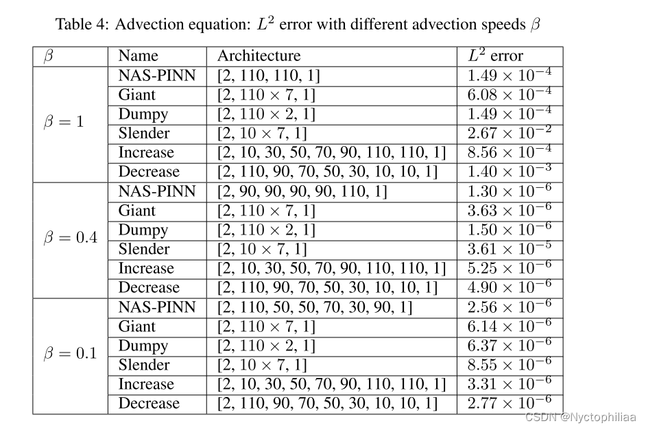
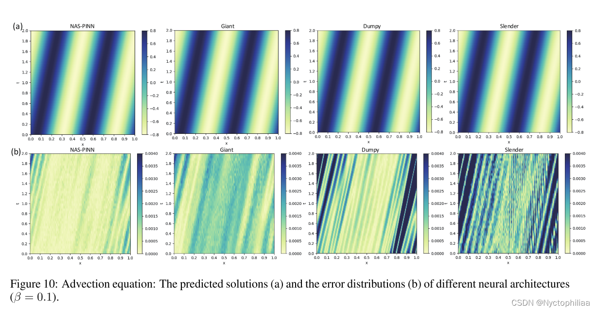
体系结构Dumpy在β = 1时性能最好，而体系结构Giant在β = 0.1时性能最好。当β = 1时，Slender架构几乎失效，但随着β的减小，结果变得更好，当β = 0.1时，Slender架构甚至可以获得与其他两种参考架构相当的结果。类似地，当β = 0.1时，体系结构的下降达到第二好的精度，但当β = 1时，得到第二差的结果。这些结果表明，面对不同的pde或条件，相同的神经结构可能会得到截然不同的效果，这给人工设计神经结构带来了麻烦，并强调了NAS研究对pnp的意义。同时， $L^{2}$ 误差表明，β越大，方程越难解。这提醒我们，复杂的问题并不总是需要深度神经网络，而相对简单的问题可能需要更多的参数来解决，这种现象进一步强调了NAS-PINN的价值。

4、结论

文章提出了一种名为NAS-PINN的神经结构搜索引导方法，用于自动搜索求解给定偏微分方程的最佳神经结构。通过构造混合运算并引入掩模来实现不同形状张量的相加，可以将结构搜索问题松弛为一个连续的双层优化问题。该方法能够在给定的搜索空间中自动搜索最合适的隐藏层数和每层的神经元数，并为特定问题构造最佳神经结构。各种数值实验验证了NAS-PINN的有效性，显示其对不规则计算域和高维问题的强适应性。

二、代码实验

考虑偏微分方程如下：

"""
A scratch for PINN solving the following PDE
u_xx-u_yyyy=(2-x^2)*exp(-y)
Author: ST
Date: 2023/2/26
"""
import torch
import matplotlib.pyplot as plt
from mpl_toolkits.mplot3d import Axes3D

epochs = 10000    # 训练代数
h = 100    # 画图网格密度
N = 1000    # 内点配置点数
N1 = 100    # 边界点配置点数
N2 = 1000    # PDE数据点

def setup_seed(seed):
    torch.manual_seed(seed)
    torch.cuda.manual_seed_all(seed)
    torch.backends.cudnn.deterministic = True

# 设置随机数种子
setup_seed(888888)

# Domain and Sampling
def interior(n=N):
    # 内点
    x = torch.rand(n, 1)
    y = torch.rand(n, 1)
    cond = (2 - x ** 2) * torch.exp(-y)
    return x.requires_grad_(True), y.requires_grad_(True), cond


def down_yy(n=N1):
    # 边界 u_yy(x,0)=x^2
    x = torch.rand(n, 1)
    y = torch.zeros_like(x)
    cond = x ** 2
    return x.requires_grad_(True), y.requires_grad_(True), cond


def up_yy(n=N1):
    # 边界 u_yy(x,1)=x^2/e
    x = torch.rand(n, 1)
    y = torch.ones_like(x)
    cond = x ** 2 / torch.e
    return x.requires_grad_(True), y.requires_grad_(True), cond


def down(n=N1):
    # 边界 u(x,0)=x^2
    x = torch.rand(n, 1)
    y = torch.zeros_like(x)
    cond = x ** 2
    return x.requires_grad_(True), y.requires_grad_(True), cond


def up(n=N1):
    # 边界 u(x,1)=x^2/e
    x = torch.rand(n, 1)
    y = torch.ones_like(x)
    cond = x ** 2 / torch.e
    return x.requires_grad_(True), y.requires_grad_(True), cond


def left(n=N1):
    # 边界 u(0,y)=0
    y = torch.rand(n, 1)
    x = torch.zeros_like(y)
    cond = torch.zeros_like(x)
    return x.requires_grad_(True), y.requires_grad_(True), cond


def right(n=N1):
    # 边界 u(1,y)=e^(-y)
    y = torch.rand(n, 1)
    x = torch.ones_like(y)
    cond = torch.exp(-y)
    return x.requires_grad_(True), y.requires_grad_(True), cond

def data_interior(n=N2):
    # 内点
    x = torch.rand(n, 1)
    y = torch.rand(n, 1)
    cond = (x ** 2) * torch.exp(-y)
    return x.requires_grad_(True), y.requires_grad_(True), cond


# Neural Network
class MLP(torch.nn.Module):
    def __init__(self):
        super(MLP, self).__init__()
        self.net = torch.nn.Sequential(
            torch.nn.Linear(2, 32),
            torch.nn.Tanh(),
            torch.nn.Linear(32, 32),
            torch.nn.Tanh(),
            torch.nn.Linear(32, 32),
            torch.nn.Tanh(),
            torch.nn.Linear(32, 32),
            torch.nn.Tanh(),
            torch.nn.Linear(32, 1)
        )

    def forward(self, x):
        return self.net(x)


# Loss
loss = torch.nn.MSELoss()


def gradients(u, x, order=1):
    if order == 1:
        return torch.autograd.grad(u, x, grad_outputs=torch.ones_like(u),
                                   create_graph=True,
                                   only_inputs=True, )[0]
    else:
        return gradients(gradients(u, x), x, order=order - 1)

# 以下7个损失是PDE损失
def l_interior(u):
    # 损失函数L1
    x, y, cond = interior()
    uxy = u(torch.cat([x, y], dim=1))
    return loss(gradients(uxy, x, 2) - gradients(uxy, y, 4), cond)


def l_down_yy(u):
    # 损失函数L2
    x, y, cond = down_yy()
    uxy = u(torch.cat([x, y], dim=1))
    return loss(gradients(uxy, y, 2), cond)


def l_up_yy(u):
    # 损失函数L3
    x, y, cond = up_yy()
    uxy = u(torch.cat([x, y], dim=1))
    return loss(gradients(uxy, y, 2), cond)


def l_down(u):
    # 损失函数L4
    x, y, cond = down()
    uxy = u(torch.cat([x, y], dim=1))
    return loss(uxy, cond)


def l_up(u):
    # 损失函数L5
    x, y, cond = up()
    uxy = u(torch.cat([x, y], dim=1))
    return loss(uxy, cond)


def l_left(u):
    # 损失函数L6
    x, y, cond = left()
    uxy = u(torch.cat([x, y], dim=1))
    return loss(uxy, cond)


def l_right(u):
    # 损失函数L7
    x, y, cond = right()
    uxy = u(torch.cat([x, y], dim=1))
    return loss(uxy, cond)

# 构造数据损失
def l_data(u):
    # 损失函数L8
    x, y, cond = data_interior()
    uxy = u(torch.cat([x, y], dim=1))
    return loss(uxy, cond)


# Training

u = MLP()
opt = torch.optim.Adam(params=u.parameters())

for i in range(epochs):
    opt.zero_grad()
    l = l_interior(u) \
        + l_up_yy(u) \
        + l_down_yy(u) \
        + l_up(u) \
        + l_down(u) \
        + l_left(u) \
        + l_right(u) \
        + l_data(u)
    l.backward()
    opt.step()
    if i % 100 == 0:
        print(i)

# Inference
xc = torch.linspace(0, 1, h)
xm, ym = torch.meshgrid(xc, xc)
xx = xm.reshape(-1, 1)
yy = ym.reshape(-1, 1)
xy = torch.cat([xx, yy], dim=1)
u_pred = u(xy)
u_real = xx * xx * torch.exp(-yy)
u_error = torch.abs(u_pred-u_real)
u_pred_fig = u_pred.reshape(h,h)
u_real_fig = u_real.reshape(h,h)
u_error_fig = u_error.reshape(h,h)
print("Max abs error is: ", float(torch.max(torch.abs(u_pred - xx * xx * torch.exp(-yy)))))
# 仅有PDE损失    Max abs error:  0.004852950572967529
# 带有数据点损失  Max abs error:  0.0018916130065917969

# 作PINN数值解图
fig = plt.figure()
ax = Axes3D(fig)
ax.plot_surface(xm.detach().numpy(), ym.detach().numpy(), u_pred_fig.detach().numpy())
ax.text2D(0.5, 0.9, "PINN", transform=ax.transAxes)
plt.show()
fig.savefig("PINN solve.png")

# 作真解图
fig = plt.figure()
ax = Axes3D(fig)
ax.plot_surface(xm.detach().numpy(), ym.detach().numpy(), u_real_fig.detach().numpy())
ax.text2D(0.5, 0.9, "real solve", transform=ax.transAxes)
plt.show()
fig.savefig("real solve.png")

# 误差图
fig = plt.figure()
ax = Axes3D(fig)
ax.plot_surface(xm.detach().numpy(), ym.detach().numpy(), u_error_fig.detach().numpy())
ax.text2D(0.5, 0.9, "abs error", transform=ax.transAxes)
plt.show()
fig.savefig("abs error.png")

实验结果：

总结

与SMAC算法的比较结果表明，NAS-PINN在更大、更灵活的搜索空间内搜索效率更高。数值结果进一步表明，更多的隐藏层并不一定意味着性能更好，有时甚至会有害。对于泊松方程和平流方程，较浅的神经网络（每层神经元较多）优于较深的神经网络，这与常识相悖。而对于汉堡方程，更多的层数对求解至关重要，即使每层神经元数量较少。实验还表明，每层有不同数量神经元的网络效果优于所有隐藏层具有相同数量神经元的网络。有效的神经架构在不同偏微分方程之间差异很大，NAS-PINN可以帮助研究这些特征，提高研究效率。未来，该方法可以应用于卷积神经网络（CNN）的搜索，自动选择DNN和CNN，并进一步研究是否保留混合层的阈值及其计算效率。