遗传算法——实现无向图聚类

GA思想

注：关于GA思想及详细步骤不再赘述，可查阅其他大牛博客
简单一句话：
物竞天择，适者生存
注：由于实战案例特殊，故未涉及基因编码、解码（十、二进制转换）以及轮盘赌算法，若感兴趣，可查阅其他大牛博客

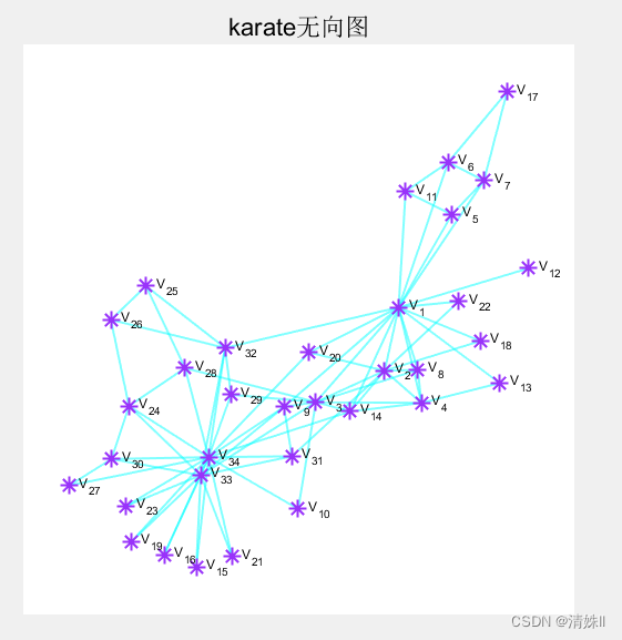
无向图聚类要求

• 将给定的无向图划分为两类点（0类和1类），使得两类点连接边最少），在本次实战中，给定34个点，0类包含n0=16个点，1类包含18个点。

GA步骤

种群初始化

• 利用randperm()函数实现种群初始化，100个种群即代表100个分类方案
  每个分类方案都必须满足16个0，18个1

% 初始种群（100个个体即100个分类方案）
p=zeros(100,n);
for i=1:100
    vector=randperm(n);
    p(i,vector>n1)=1;
end

选择

适应度函数

%计算每一个个体（分类方案）适应度
    for i=1:100
            [~,id0]=find(p(i,:)==0);
            [~,id1]=find(p(i,:)==1);
            edges=sum(sum(w(id0,id1)));
            fit(i)=1/(edges+1);
    end

计算种群平均适应度与最优适应度

%记录每次进化后的相关参数
        [pfit,index]=sort(fit,"descend");
        gen_maxp(iter)=pfit(1);
        gen_bestp(iter,:)=p(index(1),:);
        gen_meanp(iter)=mean(pfit);
        p(1:20,:)=p(index(1:20),:);%每次进化（迭代）只根据适应度大小保留前20个个体
    % 交叉—— 新产生80个个体

交叉

% 交叉—— 新产生80个个体
       num=1;
       while num<=40
              C_p=sort(randperm(34,2));
              twop=randperm(20,2);
              if sum(p(twop(1),C_p(1):C_p(2)))==sum(p(twop(2),C_p(1):C_p(2)))
                  temp=p(twop(1),C_p(1):C_p(2));
                  p(twop(1),C_p(1):C_p(2))=p(twop(2),C_p(1):C_p(2));
                  p(twop(2),C_p(1):C_p(2))=temp;
                  p(20+num,:)=p(twop(1),:);
                  p(20+num*2,:)=p(twop(2),:);
                  num=num+1;
              end
        end       

变异

   %变异
        %在经过选择，交叉后的100个个体中选择20个进行变异
        count=1;
        while count<=20
            chosep=randperm(100,20);
            [~,id0]=find(p(chosep(count),:)==0);
            [~,id1]=find(p(chosep(count),:)==1);
            p(chosep(count),id0(ceil(rand*length(id0))))=1;
            p(chosep(count),id1(ceil(rand*length(id1))))=0;
            count=count+1;
        end

完整代码

function GAgraph
%% 
clear,clc
load karate_w.mat w;
n=size(w,1);%记录图中顶点数
n1=16;%将图中顶点分为两类，0类个数为n1(16)个，1类个数为n-n1(18)个
geniter=100;
iter=1;
%为记录进化过程数组预先分配内存
gen_maxp=zeros(geniter,1);
gen_meanp=zeros(geniter,1);
gen_bestp=zeros(100,n);
 fit=zeros(100,1);
% 初始种群（100个个体即100个分类方案）
p=zeros(100,n);
for i=1:100
    vector=randperm(n);
    p(i,vector>n1)=1;
end
%% 
%种群进化
while iter<=geniter
%计算每一个个体（分类方案）适应度以及种群平均适应度与最优适应度
    for i=1:100
            [~,id0]=find(p(i,:)==0);
            [~,id1]=find(p(i,:)==1);
            edges=sum(sum(w(id0,id1)));
            fit(i)=1/(edges+1);
    end
    %记录每次进化后的相关参数
        [pfit,index]=sort(fit,"descend");
        gen_maxp(iter)=pfit(1);
        gen_bestp(iter,:)=p(index(1),:);
        gen_meanp(iter)=mean(pfit);
        p(1:20,:)=p(index(1:20),:);%每次进化（迭代）只根据适应度大小保留前20个个体
    % 交叉—— 新产生80个个体
       num=1;
       while num<=40
              C_p=sort(randperm(34,2));
              twop=randperm(20,2);
              if sum(p(twop(1),C_p(1):C_p(2)))==sum(p(twop(2),C_p(1):C_p(2)))
                  temp=p(twop(1),C_p(1):C_p(2));
                  p(twop(1),C_p(1):C_p(2))=p(twop(2),C_p(1):C_p(2));
                  p(twop(2),C_p(1):C_p(2))=temp;
                  p(20+num,:)=p(twop(1),:);
                  p(20+num*2,:)=p(twop(2),:);
                  num=num+1;
              end
        end       
        %变异
        %在经过选择，交叉后的100个个体中选择20个进行变异
        count=1;
        while count<=20
            chosep=randperm(100,20);
            [~,id0]=find(p(chosep(count),:)==0);
            [~,id1]=find(p(chosep(count),:)==1);
            p(chosep(count),id0(ceil(rand*length(id0))))=1;
            p(chosep(count),id1(ceil(rand*length(id1))))=0;
            count=count+1;
        end
      iter=iter+1;
end
[bestf,bestid]=max(gen_maxp);
bestp=gen_bestp(bestid,:);
disp('karate无向图中两类点最少连接边数：')
disp(1/bestf-1);%显示两类点最少连接边数
%找出最优个体/分类方案，以便绘图
cluster0=find(bestp==0);
cluster1=find(bestp==1);

可视化

原始无向图

注：不知如何上传karate_w.mat文件，望见谅

function PlotGraph
% 导入无向图的邻接矩阵并绘制无向图G
load karate_w.mat w
n=size(w,1);
nodes=cell(1,n);
for i=1:n
    nodes{i}=['V_{',num2str(i),'}'];
end
G=graph(w,nodes);
P=plot(G,"LineStyle","-","layout",'force',"NodeFontSize",6,...
    "Linewidth",1.0,"MarkerSize",8,"Marker","*");
P.EdgeColor='c';
P.NodeColor=[0.6,0.2,0.98];
title('karate无向图')
set(gca,'xcolor','w','ycolor','w')%不显示坐标轴
axis tight equal

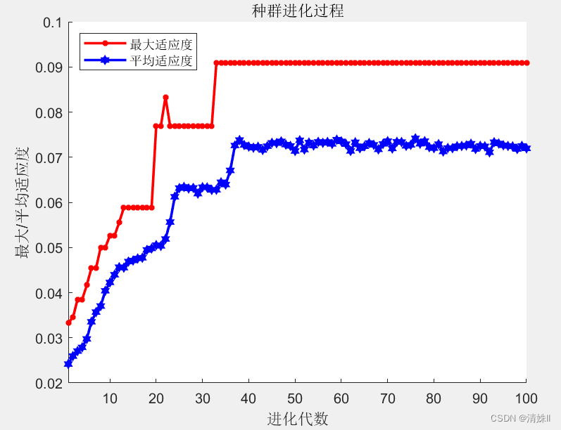
进化过程

% % 绘制运算后的适应度曲线。
% 若平均适应度与最大适应度在曲线上有趋同态势，表示算法收敛较顺利。
figure(2);  %创建序号2图窗
h1=plot(1:geniter,gen_maxp);
set(h1,'color','r','linestyle','-','linewidth',1.8,'marker','*','markersize',4)
hold on;
h2 = plot(1:geniter,gen_meanp);
set(h2,'color','b','linestyle','-','linewidth',1.8,'marker','h','markersize',4);
xlabel('进化代数');ylabel('最大/平均适应度');xlim([1 geniter]);
legend('最大适应度','平均适应度','Location','northwest');
title('种群进化过程');
box off;hold off;

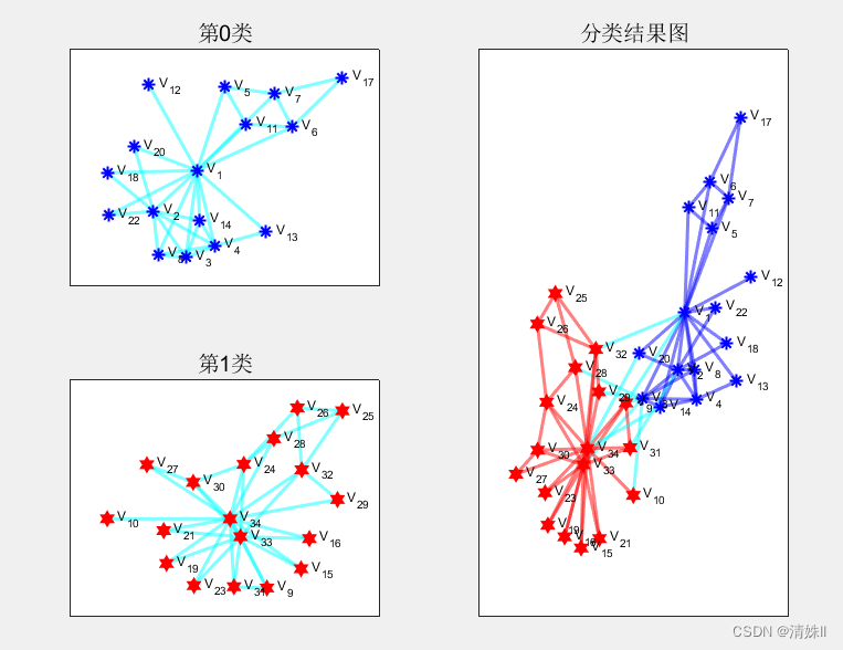
最优分类图

  function PlotBest(c0,c1)
 %绘制最好分类结果
 %分别绘制0，1类图的内部节点
load karate_w.mat w;
n=size(w,1);
nodes=cell(1,n);
n0=length(c0);
n1=length(c1);
nodes0=cell(1,n0);
nodes1=cell(1,n1);
w0=w(c0,c0);
w1=w(c1,c1);
for i=1:n
    nodes{i}=['V_{',num2str(i),'}'];
end
for i=1:n0
    nodes0{i}=['V_{',num2str(c0(i)),'}'];
end
for j=1:n1
    nodes1{j}=['V_{',num2str(c1(j)),'}'];
end
subplot(2,2,1)
G0=graph(w0,nodes0);
plot(G0,"EdgeColor",'c',"NodeColor",'b',"NodeFontSize",6,"Marker",'*',...
   "layout",'force', 'LineWidth',1.5,"MarkerSize",6);
title('第0类')
subplot(2,2,3)
G1=graph(w1,nodes1);
plot(G1,"EdgeColor",'c',"NodeColor",'r',"NodeFontSize",6,"Marker",'h',...
   "layout",'force', 'LineWidth',1.5,"MarkerSize",6);
title('第1类')
subplot(2,2,[2,4])
G=graph(w,nodes);
P=plot(G,"layout",'force',"NodeFontSize",6,...
    "Linewidth",1.5,"MarkerSize",8,"Marker",".");
P.EdgeColor='c';
P.NodeColor='k';
% 在原图基础上突出显示两类图
highlight(P,G0.Nodes.Name(:)',"NodeColor",'b',"Marker","*","MarkerSize",6)
highlight(P,G0.Edges.EndNodes(:,1)',G0.Edges.EndNodes(:,2),"EdgeColor",'b')
highlight(P,G1.Nodes.Name(:)',"NodeColor",'r',"Marker","h","MarkerSize",6)
highlight(P,G1.Edges.EndNodes(:,1)',G1.Edges.EndNodes(:,2),"EdgeColor",'r')
title('分类结果图')

结束语：写的过于简单，理解可能有些费力，建议阅读前先熟悉遗传算法原理及步骤要点，再食用本博客。