


前文对Variations-of-SFANet-for-Crowd-Counting做了一点基础梳理,链接如下:Variations-of-SFANet-for-Crowd-Counting记录-CSDN博客
本次对其中两个可视化代码进行梳理
1.Visualization_ShanghaiTech.ipynb
不太习惯用jupyter notebook, 这里改成了python代码测试,下面代码提到的测试数据都是项目自带的,权重自己下载一下吧,前文提到了一些需要下载的权重或者数据。
import warnings
warnings.filterwarnings('ignore')
import matplotlib.pyplot as plt
from matplotlib import cm as CM
import os
import numpy as np
from scipy.io import loadmat
from PIL import Image; import cv2
import torch
from torchvision import transforms
from models import M_SFANet
part = 'B'; index = 4
DATA_PATH = f"./ShanghaiTech_Crowd_Counting_Dataset/part_{part}_final/test_data/"
fname = os.path.join(DATA_PATH, "ground_truth", f"GT_IMG_{index}.mat")
img = Image.open(os.path.join(DATA_PATH, "images", f"IMG_{index}.jpg")).convert('RGB')
plt.imshow(img)
plt.gca().set_axis_off()
plt.show()
gt = loadmat(fname)["image_info"]
location = gt[0, 0][0, 0][0]
count = location.shape[0]
print(fname)
print('label:', count)
model = M_SFANet.Model()
model.load_state_dict(torch.load(f"./ShanghaitechWeights/checkpoint_best_MSFANet_{part}.pth",
map_location=torch.device('cpu'))["model"]);
trans = transforms.Compose([transforms.ToTensor(),
transforms.Normalize([0.485, 0.456, 0.406], [0.229, 0.224, 0.225])
])
height, width = img.size[1], img.size[0]
height = round(height / 16) * 16
width = round(width / 16) * 16
img = cv2.resize(np.array(img), (width,height), Image.BILINEAR)
img = trans(Image.fromarray(img))[None, :]
model.eval()
density_map, attention_map = model(img)
print('Estimated count:', torch.sum(density_map).item())
print("Visualize estimated density map")
plt.gca().set_axis_off()
plt.margins(0, 0)
plt.gca().xaxis.set_major_locator(plt.NullLocator())
plt.gca().yaxis.set_major_locator(plt.NullLocator())
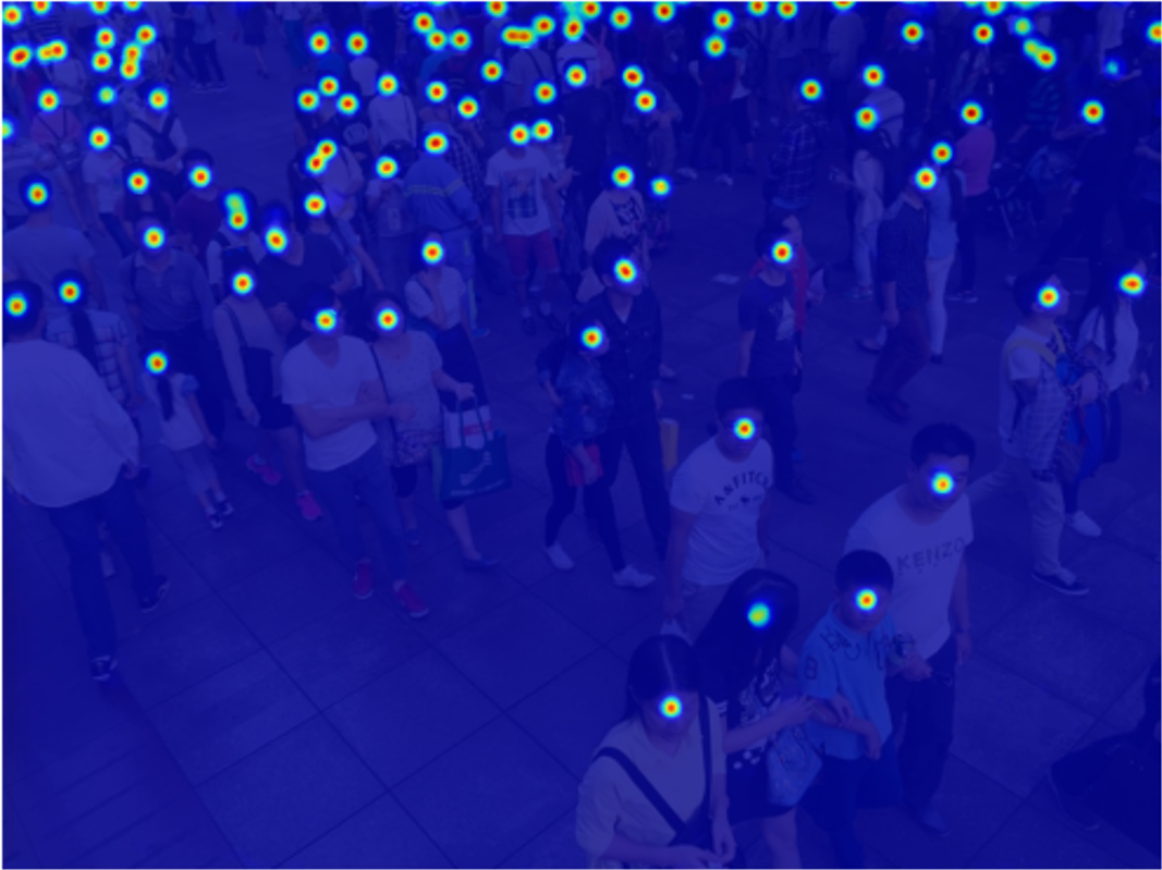
plt.imshow(density_map[0][0].detach().numpy(), cmap = CM.jet)
# plt.savefig(fname=..., dpi=300)
plt.show()运行结果如下,还有两张可视化的图


上面这样看是不是不太直观,下面这张图够直观
2.Visualization_UCF-QNRF.ipynb
同上改成了python代码测试
import torch
import os
import numpy as np
from datasets.crowd import Crowd
from models.vgg import vgg19
import argparse
from PIL import Image
import cv2
import sys
# sys.path.insert(0, '/home/pongpisit/CSRNet_keras/')
from models import M_SegNet_UCF_QNRF
from matplotlib import pyplot as plt
from matplotlib import cm as CM
datasets = Crowd(os.path.join('/home/pongpisit/CSRNet_keras/CSRNet-keras/wnet_playground/W-Net-Keras/data/UCF-QNRF_ECCV18/processed/', 'test'), 512, 8, is_gray=False, method='val')
dataloader = torch.utils.data.DataLoader(datasets, 1, shuffle=False,
num_workers=8, pin_memory=False)
model = M_SegNet_UCF_QNRF.Model()
device = torch.device('cuda')
model.to(device)
# model.load_state_dict(torch.load(os.path.join('./u_logs/0331-111426/', 'best_model.pth'), device))
model.load_state_dict(torch.load(os.path.join('./seg_logs/0327-172121/', 'best_model.pth'), device))
model.eval()
epoch_minus = []
preds = []
gts = []
for inputs, count, name in dataloader:
inputs = inputs.to(device)
assert inputs.size(0) == 1, 'the batch size should equal to 1'
with torch.set_grad_enabled(False):
outputs = model(inputs)
temp_minu = count[0].item() - (torch.sum(outputs).item())
preds.append(torch.sum(outputs).item())
gts.append(count[0].item())
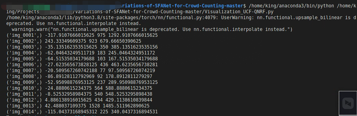
print(name, temp_minu, count[0].item(), torch.sum(outputs).item())
epoch_minus.append(temp_minu)
epoch_minus = np.array(epoch_minus)
mse = np.sqrt(np.mean(np.square(epoch_minus)))
mae = np.mean(np.abs(epoch_minus))
log_str = 'Final Test: mae {}, mse {}'.format(mae, mse)
print(log_str)
met = []
for i in range(len(preds)):
met.append(100 * np.abs(preds[i] - gts[i]) / gts[i])
idxs = []
for i in range(len(met)):
idxs.append(np.argmin(met))
if len(idxs) == 5: break
met[np.argmin(met)] += 100000000
print(set(idxs))
def resize(density_map, image):
density_map = 255*density_map/np.max(density_map)
density_map= density_map[0][0]
image= image[0]
print(density_map.shape)
result_img = np.zeros((density_map.shape[0]*2, density_map.shape[1]*2))
for i in range(result_img.shape[0]):
for j in range(result_img.shape[1]):
result_img[i][j] = density_map[int(i / 2)][int(j / 2)] / 4
result_img = result_img.astype(np.uint8, copy=False)
return result_img
def vis_densitymap(o, den, cc, img_path):
fig=plt.figure()
columns = 2
rows = 1
# X = np.transpose(o, (1, 2, 0))
X = o
summ = int(np.sum(den))
den = resize(den, o)
for i in range(1, columns*rows +1):
# image plot
if i == 1:
img = X
fig.add_subplot(rows, columns, i)
plt.gca().set_axis_off()
plt.margins(0,0)
plt.gca().xaxis.set_major_locator(plt.NullLocator())
plt.gca().yaxis.set_major_locator(plt.NullLocator())
plt.subplots_adjust(top = 1, bottom = 0, right = 1, left = 0, hspace = 0, wspace = 0)
plt.imshow(img)
# Density plot
if i == 2:
img = den
fig.add_subplot(rows, columns, i)
plt.gca().set_axis_off()
plt.margins(0,0)
plt.gca().xaxis.set_major_locator(plt.NullLocator())
plt.gca().yaxis.set_major_locator(plt.NullLocator())
plt.subplots_adjust(top = 1, bottom = 0, right = 1, left = 0, hspace = 0, wspace = 0)
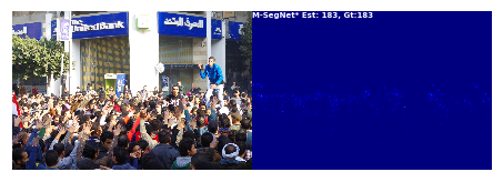
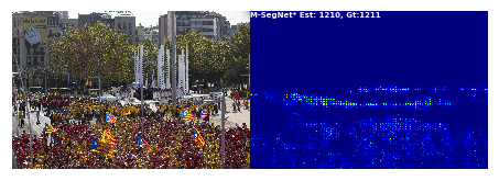
plt.text(1, 80, 'M-SegNet* Est: '+str(summ)+', Gt:'+str(cc), fontsize=7, weight="bold", color = 'w')
plt.imshow(img, cmap=CM.jet)
filename = img_path.split('/')[-1]
filename = filename.replace('.jpg', '_heatpmap.png')
print('Save at', filename)
plt.savefig('seg_'+filename, transparent=True, bbox_inches='tight', pad_inches=0.0, dpi=200)
processed_dir = '/home/pongpisit/CSRNet_keras/CSRNet-keras/wnet_playground/W-Net-Keras/data/UCF-QNRF_ECCV18/processed/test/'
model.eval()
c = 0
for inputs, count, name in dataloader:
img_path = os.path.join(processed_dir, name[0]) + '.jpg'
if c in set(idxs):
inputs = inputs.to(device)
with torch.set_grad_enabled(False):
outputs = model(inputs)
img = Image.open(img_path).convert('RGB')
height, width = img.size[1], img.size[0]
height = round(height / 16) * 16
width = round(width / 16) * 16
img = cv2.resize(np.array(img), (width,height), cv2.INTER_CUBIC)
print('Do VIS')
vis_densitymap(img, outputs.cpu().detach().numpy(), int(count.item()), img_path)
c += 1
else:
c += 1但是该代码要用UCF-QNRF_ECCV18数据集,官网的太慢了,给个靠谱的链接:UCF-QNRF_数据集-阿里云天池
下载下来,然后利用bayesian_preprocess_sh.py这个代码处理一下就可以用于上述代码了,注意一下UCF-QNRF_ECCV18的mat文件中点坐标的读取代码有点问题,自己输出一下mat文件信息就看得出来了。输出文件夹中会有相应的jpg和npy文件。

运行可视化代码,这期间遇到了一个报错
ImportError: cannot import name 'COMMON_SAFE_ASCII_CHARACTERS' from 'charset_normalizer.constant' (C:\Anaconda3\lib\site-packages\charset_normalizer\constant.py)邪门解决方案,安装一个chardet
pip install chardet -i https://pypi.tuna.tsinghua.edu.cn/simple要是上述方法还不好使就换一个,更新一下charset_normalizer,或者卸载重装charset_normalizer
pip install --upgrade charset-normalizer要是出现如下报错
RuntimeError:
        An attempt has been made to start a new process before the
        current process has finished its bootstrapping phase.

        This probably means that you are not using fork to start your
        child processes and you have forgotten to use the proper idiom
        in the main module:

            if __name__ == '__main__':
                freeze_support()
                ...

        The "freeze_support()" line can be omitted if the program
        is not going to be frozen to produce an executable.
把代码中的num_workers改成0,跑起来结果如下


 178
178


 被折叠的 条评论
为什么被折叠?
被折叠的 条评论
为什么被折叠?
 到【灌水乐园】发言


