


目录
这个案例是上石油与人工智能课程时老师给我们的一个报告题目,利用人工智能算法实现示功图的分类,并且给了我们数据集,下面我会利用五种模型(LeNet、VGG16、GoogLeNet、ResNet50和SENet)实现这个分类算法并附模型的代码,话不多说,开始吧!!!
导入相关的包
import os

import gc
# 加这俩是为了避免在训练过程中出现内存不足的情况,及时清理不必要的参数

import torch
import torch.nn as nn
import torch.nn.functional as F
import torchvision
import torchvision.transforms as transforms
import torch.optim.lr_scheduler as lr_scheduler
from torchvision.datasets import ImageFolder
from torch.utils.data import random_split
from torch.optim.optimizer import Optimizer
from torch.utils.data.dataloader import DataLoader

from tqdm import tqdm
# 用来加进度条的,方面观察模型训练的情况

from Nadam import Nadam
# 这是Nadam优化器,torch库好像没有自带的Nadam

from pyecharts.globals import CurrentConfig, NotebookType
CurrentConfig.NOTEBOOK_TYPE = NotebookType.JUPYTER_LAB
import pyecharts.options as opts
from pyecharts.charts import Line
# 绘图工具


# 导入自定义的三个模型,后面我会讲这个
from model.LeNet import LeNet
from model.VGG import VGG16
from model.GoogleNet import GoogleNet
from model.ResNet import ResNet_50
from model.SENet import SE_ResNet18
数据集展示

给的示功图数据集一共有十种,如上图所示,最终的目的就是实现这十种示功图的分类!
数据预处理
注:总的图片数量为6573张图片,并且每个类别的数量分布失衡,最低的仅87张。当你们碰到这样的情况可以考虑利用transforms.RandomCrop()、RandomHorizontalFlip()等等一系列的函数进行数据增强,老师跟我们说他给的数据集准确率可以达到99.999%,所以在这个案例中我就没有进行这个步骤啦~
对于这类的数据集,通常需要对图像进行二值化处理之后再参与模型的训练,不过当时我做这个案例的时候忘记处理这个步骤了,不过问题不大,增加了点参数量,并不影响模型的预测,后面我所构建的模型都是传入三通道类型的图片,大家可以根据需要修改即可。
这里先展示一下利用的一些包,方便大家进行案例实操;
(1)获取本地示功图数据集目录;
(2)将数据集按8:2分割成训练集和测试集(如果有需要的话可以再分出一个验证集);
(3)创建数据集加载器;
# 获取本地示功图的数据集目录
data_dir = "test_sgt"
classes = os.listdir(data_dir)
transformations = transforms.Compose([transforms.Resize((128, 128)), transforms.ToTensor()])
dataset = ImageFolder(data_dir, transform = transformations)

# 分割成训练集和测试集
train_size = int(0.8 * len(dataset))  # 训练集占总数据集的70%
test_size = len(dataset) - train_size  # 测试集大小
train_dataset, test_dataset = random_split(dataset, [train_size, test_size])

# 创建数据加载器
trainloader = DataLoader(train_dataset, batch_size=32, shuffle=True)
testloader = DataLoader(test_dataset, batch_size=32, shuffle=False)
dataset.classes
函数封装
想来想去这个模块还是写在了模型构建的前面,家人们可以简单看看写函数的作用,后面涉及到模型的时候再具体看看即可。
这个模块对模型训练测试等操作的代码进行统一的封装,主要目的就是减少代码量,毕竟每写一个模型都需要写与之对应的训练与测试的代码。
(1)模型选择与保存
"""-----定义模型保存函数-----"""
def save(model, accuracy, best_accuracy):
    if accuracy > best_accuracy:
        # 更新
        best_accuracy = accuracy
        # 保存
        torch.save(model.state_dict(), f'best_{model.__class__.__name__}.pth')
        print(f'获取到当前的最佳{model.__class__.__name__}模型参数啦!!!')
    return best_accuracy
(2)模型训练
def train(Accs, Loss, model, epoches, criterion, optimizer, scheduler):
    # 初始化准确率,用于保存最优模型参数的判别条件
    best_accuracy = 0.0

    for epoch in range(epoches):
        sum_loss = 0.0
        total = 0
        accuracy = 0.0
        for index, data in tqdm(enumerate(trainloader), total=len(trainloader), desc='Epoch {}'.format(epoch+1)):
            inputs, labels = data
            inputs, labels = inputs.to(device), labels.to(device)

            # 梯度清零
            optimizer.zero_grad()
            # 输出
            out = model(inputs)
            # Loss
            loss = criterion(out, labels)
            # 反向传播
            loss.backward()
            # 参数更新
            optimizer.step()
            # 计算准确率
            pred = torch.argmax(out, dim=1)
            total += sum([pred[i] == labels[i]  for i in range(len(pred))])

            sum_loss += loss.item()
        accuracy = total.float() / len(trainloader.dataset)
        Accs.append(round(accuracy.item(), 3))
        Loss.append(round(sum_loss / len(trainloader), 3))
        print('第{0}轮 loss: {1},识别准确率为{2}%'.format(epoch+1, sum_loss / 100, accuracy*100))
        scheduler.step()
        # 保存模型
        best_accuracy = save(model, accuracy.item(), best_accuracy)
        gc.collect()
        torch.cuda.empty_cache()
    return Accs, Loss
(3)模型测试
"""-----定义模型测试函数-----"""
def test(Accs, Finalacc, model, weight):
    model.load_state_dict(torch.load(weight))
    model.eval()

    with torch.no_grad():
        total = 0
        for index,testdata in enumerate(testloader):
            inputs, labels = testdata
            inputs, labels = inputs.to(device), labels.to(device)
            out = model(inputs)
            pred = torch.argmax(out, dim=1)
            # 计算每一批次的准确率
            tmp_total = sum([pred[i] == labels[i]  for i in range(len(pred))])
            # 计算整个测试集的准确率
            total += tmp_total
            acc = tmp_total.float()/len(pred)
            print('第{0}批次的识别准确率为{1}%'.format(index, acc*100))
            Accs.append(round(acc.item(), 3))
        Finalacc = total.float() / len(testloader.dataset)
        print('测试集的样本数量为{0}, 预测正确的个数为{1},预测准确率为{2}%'.format(len(testloader.dataset), total, Finalacc * 100))
    return Accs, Finalacc
(4)模型精调
利用随机梯度下降(SGD)对模型进行精调,本质上和上面构建的trian函数一样,只是更改了优化器;
"""-----模型精调函数-SGD-----"""
def fine(Accs, Loss, model, criterion, optimizer):
    # 初始化准确率,用于保存最优模型参数的判别条件
    best_accuracy = 0.0

    for epoch in range(50):
        sum_loss = 0.0
        total = 0
        accuracy = 0.0
        for index, data in tqdm(enumerate(trainloader), total=len(trainloader), desc='Fine Epoch {}'.format(epoch+1)):
            inputs, labels = data
            inputs, labels = inputs.to(device), labels.to(device)
            # 梯度清零
            optimizer.zero_grad()
            # 输出
            out = model(inputs)
            # Loss
            loss = criterion(out, labels)
            # 反向传播
            loss.backward()
            # 参数更新
            optimizer.step()
            # 计算准确率
            pred = torch.argmax(out, dim=1)
            total += sum([pred[i] == labels[i]  for i in range(len(pred))])

            sum_loss += loss.item()
        accuracy = total.float() / len(trainloader.dataset)
        Accs.append(round(accuracy.item(), 3))
        Loss.append(round(sum_loss / len(trainloader), 3))
        print('第{0}轮 loss: {1},识别准确率为{2}%'.format(epoch+1, sum_loss / 100, accuracy*100))
        # 保存模型
        best_accuracy = save(model, accuracy.item(), best_accuracy)
        gc.collect()
        torch.cuda.empty_cache()
    return Accs, Loss
(5)相关结果写入
这是写入模型训练和测试损失值得,写入txt文件方便后续调用作图等等;
"""-----定义训练结果存储函数-----"""
def write_to_file(filename, train_acc, train_losses, test_acc, test_final_acc):
    with open(filename, 'w') as file:
        file.write("Epoch\ttrain_Accuracy\ttrain_Loss\ttest_acc\n")
        for i in range(len(train_acc)):
            file.write(f"{i+1}\t{train_acc[i]}\t{train_losses[i]}\n")

        file.write("Epoch\ttest_Accuracy\n")
        for i in range(len(test_acc)):
            file.write(f"{i+1}\t{test_acc[i]}\n")
        file.write(f"Final_test_acc:{test_final_acc*100}%")
(6)超参数定义
构建一个超参数的字典,方便后续的调用;
hyperparameters = {
    'lr': [5e-5, 1e-4, 1e-3],  # 学习率列表
    'epochs': [20, 30, 40],  # 训练轮数
    'criterion': nn.CrossEntropyLoss(),  # 损失函数
    'optimizer': {
        'RMSprop': torch.optim.RMSprop,  # RMSprop优化器
        'SGD': torch.optim.SGD,  # 随机梯度下降优化器
        'Adam': torch.optim.Adam,  # Adam优化器
        'Nadam': Nadam,  # Nadam优化器
    },
    'scheduler': {
        'StepLR': lr_scheduler.StepLR,
        'CosineAnnealingLR': lr_scheduler.CosineAnnealingLR
    }
}
模型构建
LeNet——非常经典易懂的模型
(1)LeNet-5模型介绍
1998年,LeCun等提出LeNet-5模型,网络的基本结构为:卷积层、池化层、全连接层。基于LeNet-5模型对示功图分类,建立深度为7层的网络结构。如图下图所示,主要包括两个特征提取层、全连接层、输出层。其中特征提取层包括一个卷积层和池化层。

(2)LeNet-5模型改动
参照LeNet-5模型结构,设置卷积核大小为3×3,设置三个卷积层,三个卷积层对应的卷积核数量分别设为64、256和128。池化层选择的窗口尺寸为2×2,步长设为2。采用最大池化方式,降低信息的冗余,提取图像的显著特征。参数对应每个卷积层的卷积核数量,在每个池化层之后增加BatchNorm2d层,全连接层增加两层,其他结构参数不变。模型的输入图片大小为128×128,输入层预处理后将数据转化为统一格式,使用Adam优化器更新网络权重。
小贴士:可以根据实际需要更改层数、卷积核大小和个数等等。
(3)LeNet模型代码
| LeNet超参数 | 取值 |
| 学习率 | 5e-5 |
| 迭代次数 | 20 |
| 损失函数 | CrossEntropyLoss |
| 优化器 | Adam |
| 学习率调度器 | StepLR |
import torch
import torch.nn as nn

# 定义LeNet神经网络
class LeNet(nn.Module):
    def __init__(self):
        super(LeNet, self).__init__()
        # 参数解释:nn.Conv2d(in_channels, out_channels, kernel_size, stride, padding)
        # 第一个卷积层,
        self.conv = nn.Sequential(
            nn.Conv2d(3, 64, 5, 1),#124
            nn.ReLU(),
            nn.MaxPool2d(2, 2), # 62
            # 加入正则化项
            nn.BatchNorm2d(64),

            # 第二个卷积层
            nn.Conv2d(64, 256, 3, 1), # 60
            nn.ReLU(),
            nn.MaxPool2d((2,2)), # 30
            nn.BatchNorm2d(256),

            # 第三个卷积层
            nn.Conv2d(256, 128, 3, 1),#28
            nn.ReLU(),
            nn.MaxPool2d((2,2)),#14
            nn.BatchNorm2d(128)
        )

        self.fc = nn.Sequential(
            nn.Linear(128*14*14, 2500),
            nn.ReLU(),
            nn.Linear(2500, 1200),
            nn.ReLU(),
            nn.Linear(1200, 200),
            nn.ReLU(),
            nn.Linear(200, 10)
        )
    def forward(self, x):
        x = self.conv(x)
        out = self.fc(x.view(x.size(0), -1))

        # 加入softmax分类器
        classifer = nn.Softmax(dim=0)
        out = classifer(out)

        return out
LeNet模型训练:
"""-----模型训练-----"""
# 模型实例化
Lenet = LeNet().to(device)
# 学习率
lr = hyperparameters['lr'][0]
# 迭代次数
epoches = hyperparameters['epochs'][0]
# 损失函数
criterion = hyperparameters['criterion']
# 优化器
optimizer = hyperparameters['optimizer']['Adam'](Lenet.parameters(), lr=lr)
# 学习率调度器
lr_decay = 0.9
step_size = 10
scheduler = hyperparameters['scheduler']['StepLR'](optimizer, step_size=step_size, gamma=lr_decay)
# 训练
# 初始化准确值,损失值保存链表
accLeNet = []
lossLeNet = []
accLeNet, lossLeNet = train(accLeNet, lossLeNet, Lenet, epoches, criterion, optimizer, scheduler)
LeNet模型测试:
"""-----测试-----"""
weights = "best_LeNet.pth"
# 每个批次的测试准确率与
testLeNet, FinalLeNet = [], 0.0
# 模型测试
testLeNet, FinalLeNet = test(testLeNet, FinalLeNet, Lenet, weights)
# 写入txt文件,方便后续调用作图
write_to_file('LeNet.txt', accLeNet, lossLeNet, testLeNet, FinalLeNet)
(4)效果展示

对于修改的LeNet模型,设置的总迭代次数为20次,在第17次的模型训练时预测准确率达到了98.82%,测试阶段通过load函数加载best_LeNet.pth进行模型的测试,最终的测试准确率达到了97.64%,预测正确的样本个数为1284个(测试集的总样本个数为1315)。


VGG16——小卷积池化核
(1)VGG16 模型介绍
VGG16 是一种深度卷积神经网络(CNN)模型,由牛津大学的 Visual Geometry Group (VGG) 开发。这个模型在 2014 年的 ImageNet Large Scale Visual Recognition Challenge (ILSVRC) 竞赛中取得了显著的成绩。
VGG16包含 16 个权重层(卷积层和全连接层)。权重层使用多个 3x3 的小卷积核来替代较大卷积核(如 5x5 或 7x7),这种设计使得网络可以学习更复杂的模式,同时减少参数的数量。VGG16 中的卷积层是成组堆叠的,每组中的卷积层具有相同的卷积核大小。这些组之间通过最大池化层进行连接,以减小特征图的空间尺寸并增加感受野。在卷积层之后,VGG16 包含三个全连接层,用于将卷积层提取的特征映射到最终的分类空间。
(2)VGG16模型代码
| VGG16超参数 | 取值 |
| 学习率 | 1e-4 |
| 迭代次数 | 20 |
| 损失函数 | CrossEntropyLoss |
| 优化器 | Adam |
| 学习率调度器 | CosineAnnealingLR |
import torch
import torch.nn.functional as F
import torch.nn as nn
# 定义VGG块
def vgg_block(in_channels, out_channels, num_conv_layers):
    layers = []
    for _ in range(num_conv_layers):
        layers.append(nn.Conv2d(in_channels, out_channels, kernel_size=3, padding=1))
        layers.append(nn.ReLU(inplace=True))
        in_channels = out_channels
    layers.append(nn.MaxPool2d(kernel_size=2, stride=2))
    return nn.Sequential(*layers)

"""
    定义VGG网络
"""
class VGG16(nn.Module):
    def __init__(self, num_classes=10):
        super(VGG16, self).__init__()
        self.features = nn.Sequential(
            vgg_block(3, 64, 2),    # 2个卷积层,64个输出通道----64
            nn.BatchNorm2d(64),
            vgg_block(64, 128, 2),  # 2个卷积层,128个输出通道---32
            nn.BatchNorm2d(128),
            vgg_block(128, 256, 3), # 3个卷积层,256个输出通道---16
            nn.BatchNorm2d(256),
            vgg_block(256, 512, 3), # 3个卷积层,512个输出通道---8
            nn.BatchNorm2d(512),
            vgg_block(512, 512, 3)  # 3个卷积层,512个输出通道---4
        )
        self.classifier = nn.Sequential(
            nn.Linear(512 * 4 * 4, 4096),
            nn.ReLU(inplace=True),
            nn.Dropout(),
            nn.Linear(4096, 4096),
            nn.ReLU(inplace=True),
            nn.Dropout(),
            nn.Linear(4096, num_classes)
        )

    def forward(self, x):
        x = self.features(x)
        x = torch.flatten(x, 1)
        x = self.classifier(x)
        return x
VGG16模型训练:
"""-----模型训练-----"""
# 模型实例化
Vgg = VGG16().to(device)
# 学习率
lr = hyperparameters['lr'][1]
# 迭代次数
epoches = hyperparameters['epochs'][0]
# 损失函数
criterion = hyperparameters['criterion']
# 优化器
optimizer = hyperparameters['optimizer']['Adam'](Vgg.parameters(), lr=lr)
# 学习率调度器
scheduler = hyperparameters['scheduler']['CosineAnnealingLR'](optimizer, T_max=10)
# 训练
# 初始化准确值,损失值保存链表
accVgg = []
lossVgg = []
accVgg, lossVgg = train(accVgg, lossVgg, Vgg, epoches, criterion, optimizer, scheduler)
VGG16模型测试:
"""-----测试-----"""
weights = "best_VGG16.pth"
# 每个批次的测试准确率与
testVgg, FinalVgg = [], 0.0
# 模型测试
testVgg, FinalVgg = test(testVgg, FinalVgg, Vgg, weights)
# 写入txt文件,方便后续调用作图
write_to_file('VGG16.txt', accVgg, lossVgg, testVgg, FinalVgg)
(3)效果展示

VGG16模型作为经典的神经网络模型,在第11次迭代预测准确率就达到了99.96%(作图显示100%是保留3位小数四舍五入得到),通过save函数保存了这一迭代更新的参数,在后续测试过程中预测正确的样本个数达到了1311个,预测准确率为99.695%,由于测试集也是按32的批次大小参与模型预测,几乎所有的批次都达到了100%的预测准确率!


GoogLeNet——Inception模块
(1)GoogLeNet模型介绍
GoogLeNet,也称为Inception网络,是由Google研究团队在2014年提出的一种深度卷积神经网络架构。它是当时ImageNet大规模视觉识别竞赛中取得重要突破的一个关键模型。
GoogLeNet的主要特点是其极深的网络结构和高效的计算。与传统的深度神经网络相比,GoogLeNet采用了一种称为Inception模块的特殊设计,可以在减少参数数量的同时增加网络深度和宽度,从而提高了模型的识别性能。此外,GoogLeNet还采用了全局平均池化和多个辅助分类器等技术来加速训练和降低过拟合风险。
(2)Inception模块
GoogLeNet最突出的特点之一就是采用了Inception模块。Inception模块采用了一种多分支结构,包含了不同大小的卷积核和池化核,以及不同尺度的特征图。通过这种多分支结构,Inception模块可以在保持计算量相对较低的情况下,提取更丰富的特征信息。

(3)GoogLeNet模型代码
| GoogLeNet超参数 | 取值 |
| 学习率 | 1e-4 |
| 迭代次数 | 20 |
| 损失函数 | CrossEntropyLoss |
| 优化器 | Adam |
| 学习率调度器 | StepLR |
import torch
import torch.nn.functional as F
import torch.nn as nn

"""
    Inception模块的基本组成结构有四个:1x1卷积,3x3卷积,5x5卷积,3x3最大池化
    其中3*3卷积和5*5卷积均在1*1卷积之后;3*3最大池化在1*1卷积之前
"""
# 定义Inception模块
class Inception(nn.Module):
    def __init__(self, in_channels, out_1, in_3, out_3, in_5, out_5, out_pool):
        super(Inception, self).__init__()

        # 1 * 1的卷积
        self.branch_1 = nn.Sequential(
            nn.Conv2d(in_channels, out_1, kernel_size=1),
            nn.ReLU(inplace=True)
        )

        # 3 * 3的卷积
        self.branch_3 = nn.Sequential(
            nn.Conv2d(in_channels, in_3, kernel_size=1),
            nn.ReLU(inplace=True),
            nn.Conv2d(in_3, out_3, kernel_size=3, padding=1),
            nn.ReLU(inplace=True)
        )

        # 5 * 5的卷积
        self.branch_5 = nn.Sequential(
            nn.Conv2d(in_channels, in_5, kernel_size=1),
            nn.ReLU(inplace=True),
            nn.Conv2d(in_5, out_5, kernel_size=5, padding=2),
            nn.ReLU(inplace=True)
        )

        # 3 * 3的池化
        self.MaxPool = nn.Sequential(
            nn.MaxPool2d(kernel_size=3, stride=1, padding=1),
            nn.Conv2d(in_channels, out_pool, kernel_size=1),
            nn.ReLU(inplace=True)
        )

    def forward(self, x):
        branch1_out = self.branch_1(x)
        branch3_out = self.branch_3(x)
        branch5_out = self.branch_5(x)
        MaxPool_out = self.MaxPool(x)

        out = [branch1_out, branch3_out, branch5_out, MaxPool_out]

        return torch.cat(out, 1)

class GoogleNet(nn.Module):
    def __init__(self, num_classes=10):
        super(GoogleNet, self).__init__()

        # 前面几层
        self.Conv1 = nn.Conv2d(3, 64, kernel_size=7, stride=2, padding=3)
        self.Maxpool1 = nn.MaxPool2d(kernel_size=3, stride=2, padding=1)

        self.Conv2 = nn.Conv2d(64, 64, kernel_size=1)
        self.Conv3 = nn.Conv2d(64, 192, kernel_size=3, padding=1)
        self.Maxpool2 = nn.MaxPool2d(kernel_size=3, stride=2, padding=1)

        # inception层
        # 第一个
        self.inception3a = Inception(192, 64, 96, 128, 16, 32, 32)
        self.inception3b = Inception(256, 128, 128, 192, 32, 96, 64)
        self.Maxpool3 = nn.MaxPool2d(kernel_size=3, stride=2, padding=1)

        # 第二个
        self.inception4a = Inception(480, 192, 96, 208, 16, 48, 64)
        self.inception4b = Inception(512, 160, 112, 224, 24, 64, 64)
        self.inception4c = Inception(512, 128, 128, 256, 24, 64, 64)
        self.inception4d = Inception(512, 112, 144, 288, 32, 64, 64)
        self.inception4e = Inception(528, 256, 160, 320, 32, 128, 128)
        self.Maxpool4 = nn.MaxPool2d(kernel_size=3, stride=2, padding=1)

        # 第三个
        self.inception5a = Inception(832, 256, 160, 320, 32, 128, 128)
        self.inception5b = Inception(832, 384, 192, 384, 48, 128, 128)

        # 全局平均池化
        self.Avgpool = nn.AdaptiveAvgPool2d((1,1))
        self.dropout = nn.Dropout(0.4)
        self.fc = nn.Linear(1024, num_classes)

    def forward(self, x):
        Conv1_out = self.Maxpool1(F.relu(self.Conv1(x)))
        Conv2_out = F.relu(self.Conv2(Conv1_out))
        Conv3_out = self.Maxpool2(F.relu(self.Conv3(Conv2_out)))

        # inception层
        out = self.inception3a(Conv3_out)
        out = self.inception3b(out)
        out = self.Maxpool3(out)

        out = self.inception4a(out)
        out = self.inception4b(out)
        out = self.inception4c(out)
        out = self.inception4d(out)
        out = self.inception4e(out)
        out = self.Maxpool4(out)

        out = self.inception5a(out)
        out = self.inception5b(out)

        # 全局平均池化
        out = self.Avgpool(out)
        out = torch.flatten(out, 1)
        out = self.dropout(out)
        out = self.fc(out)

        return out
GoogLeNet模型训练:
"""-----模型训练-----"""
# 模型实例化
Googlenet = GoogleNet().to(device)
# 学习率
lr = hyperparameters['lr'][1]
# 迭代次数
epoches = hyperparameters['epochs'][0]
# 损失函数
criterion = hyperparameters['criterion']
# 优化器
optimizer = hyperparameters['optimizer']['Adam'](Googlenet.parameters(), lr=lr)
# 学习率调度器
lr_decay = 0.9
step_size = 10
scheduler = hyperparameters['scheduler']['StepLR'](optimizer, step_size=step_size, gamma=lr_decay)
# 训练
# 初始化准确值,损失值保存链表
accGoogle = []
lossGoogle = []
accGoogle, lossGoogle = train(accGoogle, lossGoogle, Googlenet, epoches, criterion, optimizer, scheduler)
GoogLeNet模型测试:
"""-----测试-----"""
weights = "best_GoogleNet.pth"
# 每个批次的测试准确率与
testGoogle, FinalGoogle = [], 0.0
# 模型测试
testGoogle, FinalGoogle = test(testGoogle, FinalGoogle, Googlenet, weights)
# 写入txt文件,方便后续调用作图
write_to_file('GoogLeNet.txt', accGoogle, lossGoogle, testGoogle, FinalGoogle)
(4)效果展示

利用GoogLeNet网络模型训练时,在第20次迭代达到最高的准确率99.83%,同样利用save保存此时的权重,在后续用于测试集预测时预测正确的样本达到了1307个,预测准确率为99.39%

ResNet50 ——残差结构
(1) ResNet50模型介绍
ResNet50是一个深度残差网络,具有50层的深度,由微软研究院的Kaiming He等人于2015年提出。ResNet50是ResNet系列中的一种,通过残差连接解决了深度神经网络中的梯度消失和梯度爆炸问题,使得网络可以更深地学习特征表示,是其较为简单的变体之一。
(2)残差模块
ResNet50的核心是残差连接,它解决了深度神经网络中出现的梯度消失和梯度爆炸问题。残差连接通过将输入直接加到网络的某些层的输出上,使得网络可以学习到残差,即网络需要学习的部分,从而更容易地训练出非常深的网络。

ResNet50主要由一系列残差块组成。每个残差块包含两个分支,一个是恒等映射分支,另一个是残差映射分支。恒等映射分支直接将输入传递到输出,而残差映射分支通过一系列卷积层来学习残差,并将学习到的残差与输入相加,得到最终的输出。
(3)ResNet50模型代码
| ResNet50超参数 | 取值 |
| 学习率 | 1e-4 |
| 迭代次数 | 20 |
| 损失函数 | CrossEntropyLoss |
| 优化器 | RMSprop |
| 学习率调度器 | StepLR |
import torch
import torch.nn.functional as F
import torch.nn as nn

"""
    定义BasicBlock模块---适用于18-layer、 34-layer
"""
class Basic_block(nn.Module):
    expansion = 1
    def __init__(self, inchannel, outchannel, stride=1):
        super(Basic_block, self).__init__()

        self.conv1 = nn.Conv2d(inchannel, outchannel, kernel_size=3,
                               stride=stride, padding=1, bias=False)
        self.bn1 = nn.BatchNorm2d(outchannel)

        self.conv2 = nn.Conv2d(outchannel, outchannel, kernel_size=3,
                               stride=1, padding=1, bias=False)
        self.bn2 = nn.BatchNorm2d(outchannel)

        self.shortcut =  nn.Sequential()
        if stride !=1 or inchannel != self.expansion*outchannel:
            self.shortcut = nn.Sequential(
                nn.Conv2d(inchannel, self.expansion*outchannel,
                         kernel_size=1, stride=stride, bias=False),
                nn.BatchNorm2d(self.expansion*outchannel)
            )
    def forward(self, x):
        out = F.relu(self.bn1(self.conv1(x)))
        out = self.bn2(self.conv2(out))
        out += self.shortcut(x)
        out = F.relu(out)

        return out

"""
    定义Bottleneck模块---适用于50-layer、 101-layer、152-layer
"""
class Bottle_neck(nn.Module):
    expansion = 4
    def __init__(self, inchannel, outchannel, stride=1):
        super(Bottle_neck, self).__init__()
        self.conv1 = nn.Conv2d(inchannel, outchannel, kernel_size=1,
                               stride=1, bias=False)
        self.bn1 = nn.BatchNorm2d(outchannel)

        self.conv2 = nn.Conv2d(outchannel, outchannel, kernel_size=3,
                              stride=stride, padding=1, bias=False)
        self.bn2 = nn.BatchNorm2d(outchannel)

        self.conv3 = nn.Conv2d(outchannel, self.expansion*outchannel, kernel_size=1,
                              stride=1, bias=False)
        self.bn3 = nn.BatchNorm2d(self.expansion*outchannel)

        self.shortcut = nn.Sequential()

        if stride != 1 or inchannel != self.expansion * outchannel:
            self.shortcut = nn.Sequential(
                nn.Conv2d(inchannel, self.expansion * outchannel, kernel_size=1,
                         stride=stride, bias=False),
                nn.BatchNorm2d(self.expansion*outchannel)
            )
    def forward(self, x):
        out = F.relu(self.bn1(self.conv1(x)))
        out = F.relu(self.bn2(self.conv2(out)))
        out = self.bn3(self.conv3(out))
        out += self.shortcut(x)
        out = F.relu(out)

        return out

'''----搭建ResNet结构-----'''
class ResNet(nn.Module):
    def __init__(self, block, num_blocks, num_classes=10):
        # block 基本块(BasicBlock or BottleBolck)  num_blocks 包含四个整数,表示每个阶段的基本块数量
        super(ResNet, self).__init__()
        self.in_planes = 64

        self.conv1 = nn.Conv2d(3, 64, kernel_size=3,
                               stride=1, padding=1, bias=False)                  # conv1

        self.bn1 = nn.BatchNorm2d(64)

        self.layer1 = self._make_layer(block, 64,  num_blocks[0], stride=1)      # conv2_x
        self.layer2 = self._make_layer(block, 128, num_blocks[1], stride=2)      # conv3_x
        self.layer3 = self._make_layer(block, 256, num_blocks[2], stride=2)      # conv4_x
        self.layer4 = self._make_layer(block, 512, num_blocks[3], stride=2)      # conv5_x

        self.avgpool = nn.AdaptiveAvgPool2d((1, 1))

        self.linear = nn.Linear(512 * block.expansion, num_classes)

    def _make_layer(self, block, planes, num_blocks, stride):
        strides = [stride] + [1]*(num_blocks-1)
        layers = []#存入每一个block
        for stride in strides:
            layers.append(block(self.in_planes, planes, stride))
            self.in_planes = planes * block.expansion

        return nn.Sequential(*layers)

    def forward(self, x):
        x = F.relu(self.bn1(self.conv1(x)))
        x = self.layer1(x)
        x = self.layer2(x)
        x = self.layer3(x)
        x = self.layer4(x)
        x = self.avgpool(x)
        # 降维
        x = torch.flatten(x, 1)

        out = self.linear(x)

        return out

def ResNet_18():
    return ResNet(Basic_block, [2, 2, 2, 2], 10)

def ResNet_34():
    return ResNet(Basic_block, [3, 4, 6, 3], 10)

def ResNet_50():
    return ResNet(Bottle_neck, [3, 4, 6, 3], 10)

def ResNet_101():
    return ResNet(Bottle_neck, [3, 4, 23, 3], 10)

def ResNet_152():
    return ResNet(Bottle_neck, [3, 8, 36, 3], 10)
ResNet50模型训练:
"""-----模型训练-----"""
# 模型实例化
ResNet50 = ResNet_50().to(device)
# 学习率
lr = hyperparameters['lr'][1]
# 迭代次数
epoches = hyperparameters['epochs'][0]
# 损失函数
criterion = hyperparameters['criterion']
# 优化器
optimizer = hyperparameters['optimizer']['RMSprop'](ResNet50.parameters(), lr=lr)
# 学习率调度器
lr_decay = 0.9
step_size = 10
scheduler = hyperparameters['scheduler']['StepLR'](optimizer, step_size=step_size, gamma=lr_decay)
# 训练
accResnet = []
lossResnet = []
accResnet, lossResnet = train(accResnet, lossResnet, ResNet50, epoches, criterion, optimizer, scheduler)
ResNet50模型测试:
"""-----测试-----"""
weights = "best_ResNet.pth"
# 每个批次的测试准确率与
testResnet, FinalResnet = [], 0.0
# 模型测试
testResnet, FinalResnet = test(testResnet, FinalResnet, ResNet50, weights)
# 写入txt文件,方便后续调用作图
write_to_file('ResNet50.txt', accResnet, lossResnet, testResnet, FinalResnet)
(4) 效果展示

ResNet50通过第一次训练准确率就达到85.6%,在这一点上比其他四个模型都要好,在第14次迭代训练集准确率达到了99.92%,在测试集上的准确率为99.54%,预测正确的样本个数为1309个。


SENet——SE模块
(1)SE模块介绍
SE模块是深度学习中用于改进卷积神经网络性能的一种技术,最早由JieHu等人在2017年提出。该模块的主要目的是增强神经网络对不同通道的特征权重的关注,使其能够更加智能地提取重要特征,从而提高模型的性能。
SE模块的核心思想是通过学习通道之间的相关性来调整每个通道的重要性,它通过一下三步实现这一目标:
第一步:压缩。 SE模块对输入特征图进行全局平均池化,得到每个通道的全局信息。全局平均池化通过在每个通道上对所有空间位置求平均值,产生一个包含每个通道信息的向量。
第二步:激活。SE模块利用两个全连接层,分别用于降维和升维。这个网络会对先前步骤得到的向量进行操作,生成一组权重,这些权重用于调整每个通道的重要性,激活函数通常是ReLU和Sigmoid。
第三步:缩放。SE模块将通过激活步骤得到的权重向量应用于原始输入特征图,通过逐元素相乘的方式对每个通道进行缩放。这一过程将增强重要的通道,同时抑制不那么重要的通道,从而使网络更关注具有显著信息的通道。

(2)SEResNet18代码
在SE模块介绍中说明,SE模块是用来改进模型性能的一种技术,它能够嵌入DeneNet系列、ResNetXt系列等等,为了方便代码的书写,因此直接利用了上面写好的ResNet模型,增加了SE模块。
注:鉴于为什么将SE模块嵌入ResNet18而不用更深的ResNet50、ResNet101或者ResNet152,主要与电脑的显存有关,如果模型的参数量太大,模型可能连初始化都不能完成,而且在模型训练过程中会有很多冗余的参数,他们一样消耗显存,很可能导致模型刚训练一会就因为内存不足就被迫终止了,这也是我亲身经历的事情,有一说一真的很难受,所以import gc就是这样来的,建议大家在训练模型之前也导入这个包写一下相关的函数!!!
| SEResNet18超参数 | 取值 |
| 学习率 | 1e-4 |
| 迭代次数 | 20 |
| 损失函数 | CrossEntropyLoss |
| 优化器 | Adam |
| 学习率调度器 | StepLR |
import torch
import torch.nn as nn
import torch.nn.functional as F

# 定义SE模块
class SE_block(nn.Module):
    def __init__(self, inchannel, ratio=16):
        super(SE_block, self).__init__()
        # 全局平均池化
        self.gap = nn.AdaptiveAvgPool2d((1,1))
        # 定义两个全连接层
        self.fc = nn.Sequential(
            nn.Linear(inchannel, inchannel // ratio, bias=False),
            nn.ReLU(),
            nn.Linear(inchannel // ratio, inchannel, bias=False),
            nn.Sigmoid()
        )
    def forward(self, x):
        b, c, h, w = x.size()
        # 池化
        y = self.gap(x).view(b, c)
        # 全连接
        y = self.fc(y).view(b, c, 1, 1)
        # 加权
        return x * y.expand_as(x)

# 将SE模块加入到BasicBlock模块中,这个模块有两种类型,一个残差分支上没有卷积,一个有卷积
# 适用于18-layer、 34-layer
class Basic_block(nn.Module):
    expansion = 1

    def __init__(self, inchannel, outchannel, stride=1):
        super(Basic_block, self).__init__()

        self.conv1 = nn.Conv2d(inchannel, outchannel, kernel_size=3,
                               stride=stride, padding=1, bias=False)
        self.bn1 = nn.BatchNorm2d(outchannel)

        self.conv2 = nn.Conv2d(outchannel, outchannel, kernel_size=3,
                               stride=1, padding=1, bias=False)
        self.bn2 = nn.BatchNorm2d(outchannel)

        self.SE = SE_block(outchannel)

        self.shortcut =  nn.Sequential()
        if stride !=1 or inchannel != self.expansion*outchannel:
            self.shortcut = nn.Sequential(
                nn.Conv2d(inchannel, self.expansion*outchannel,
                         kernel_size=1, stride=stride, bias=False),
                nn.BatchNorm2d(self.expansion*outchannel)
            )
    def forward(self, x):
        out = F.relu(self.bn1(self.conv1(x)))
        out = self.bn2(self.conv2(out))
        SE_out = self.SE(out)
        out = out * SE_out
        out += self.shortcut(x)
        out = F.relu(out)

        return out

# 将SE模块加入到BottleNeck模块中,也有两种类型,和上面的一样
# 适用于50-layer、 101-layer、152-layer
class Bottle_neck(nn.Module):
    expansion = 4

    def __init__(self, inchannel, outchannel, stride=1):
        super(Bottle_neck, self).__init__()
        self.conv1 = nn.Conv2d(inchannel, outchannel, kernel_size=1,
                               stride=1, bias=False)
        self.bn1 = nn.BatchNorm2d(outchannel)

        self.conv2 = nn.Conv2d(outchannel, outchannel, kernel_size=3,
                              stride=stride, padding=1, bias=False)
        self.bn2 = nn.BatchNorm2d(outchannel)

        self.conv3 = nn.Conv2d(outchannel, self.expansion*outchannel, kernel_size=1,
                              stride=1, bias=False)
        self.bn3 = nn.BatchNorm2d(self.expansion*outchannel)

        self.SE = SE_block(self.expansion*outchannel)

        self.shortcut = nn.Sequential()

        if stride != 1 or inchannel != self.expansion * outchannel:
            self.shortcut = nn.Sequential(
                nn.Conv2d(inchannel, self.expansion * outchannel, kernel_size=1,
                         stride=stride, bias=False),
                nn.BatchNorm2d(self.expansion*outchannel)
            )
    def forward(self, x):
        out = F.relu(self.bn1(self.conv1(x)))
        out = F.relu(self.bn2(self.conv2(out)))
        out = self.bn3(self.conv3(out))
        SE_out = self.SE(out)
        out = out * SE_out
        out += self.shortcut(x)
        out = F.relu(out)

        return out

'''-----四、搭建SE_ResNet结构-----'''
class SE_ResNet(nn.Module):
    def __init__(self, block, num_blocks, num_classes=10):
        # block 基本块(BasicBlock or BottleBolck)  num_blocks 包含四个整数,表示每个阶段的基本块数量
        super(SE_ResNet, self).__init__()
        self.in_planes = 64

        self.conv1 = nn.Conv2d(3, 64, kernel_size=3,
                               stride=1, padding=1, bias=False)                  # conv1

        self.bn1 = nn.BatchNorm2d(64)

        self.layer1 = self._make_layer(block, 64,  num_blocks[0], stride=1)      # conv2_x
        self.layer2 = self._make_layer(block, 128, num_blocks[1], stride=2)      # conv3_x
        self.layer3 = self._make_layer(block, 256, num_blocks[2], stride=2)      # conv4_x
        self.layer4 = self._make_layer(block, 512, num_blocks[3], stride=2)      # conv5_x

        self.avgpool = nn.AdaptiveAvgPool2d((1, 1))

        self.linear = nn.Linear(512 * block.expansion, num_classes)

    def _make_layer(self, block, planes, num_blocks, stride):
        strides = [stride] + [1]*(num_blocks-1)
        layers = []#存入每一个block
        for stride in strides:
            layers.append(block(self.in_planes, planes, stride))
            self.in_planes = planes * block.expansion

        return nn.Sequential(*layers)

    def forward(self, x):
        x = F.relu(self.bn1(self.conv1(x)))
        x = self.layer1(x)
        x = self.layer2(x)
        x = self.layer3(x)
        x = self.layer4(x)
        x = self.avgpool(x)
        # 降维
        x = torch.flatten(x, 1)

        out = self.linear(x)

        return out

def SE_ResNet18():
    return SE_ResNet(Basic_block, [2, 2, 2, 2])
SEResNet18模型训练:
"""-----模型训练-----"""
# 模型实例化
SENet = SE_ResNet18().to(device)
# 学习率
lr = hyperparameters['lr'][1]
# 迭代次数
epoches = hyperparameters['epochs'][0]
# 损失函数
criterion = hyperparameters['criterion']
# 优化器
optimizer = hyperparameters['optimizer']['Adam'](SENet.parameters(), lr=lr)
# 学习率调度器
lr_decay = 0.9
step_size = 10
scheduler = hyperparameters['scheduler']['StepLR'](optimizer, step_size=step_size, gamma=lr_decay)
# 训练
accSEnet = []
lossSEnet = []
accSEnet, lossSEnet = train(accSEnet, lossSEnet, SENet, epoches, criterion, optimizer, scheduler)
SEResNet18模型测试:
"""-----测试-----"""
weights = "best_SE_ResNet.pth"
testSEnet, FinalSEnet = [], 0.0
# 模型测试
testSEnet, FinalSEnet = test(testSEnet, FinalSEnet, SENet, weights)
# 写入txt文件,方便后续调用作图
write_to_file('SEResNet18.txt', accSEnet, lossSEnet, testSEnet, FinalSEnet)
(3)效果展示

通过引入SE模块改进ResNet残差网络,同时结合参数量的大小与电脑性能原因,最终选取了将SE模块融入ResNet18残差网络。
SEResNet18网络在第18轮迭代达到99.94%的准确率,在测试集上同样表现优秀,预测准确率达到了99.61%,预测正确的样本个数为1310个。


模型分析
本项目利用五个算法模型对示功图进行了分类。考虑训练集的预测准确率与损失值变化,VGG16以微弱的差距优势取得了第一,在第11次就达到了最高的准确率99.96%(经四舍五入后作图显示为1),相比与其他四个模型准确率最高;同时,在第一步迭代时,VGG16就展现了强大的模型预测能力,仅通过一步迭代达到了准确率就达到了80.3%,明显优于GoogLeNet模型和SEResNet18模型。
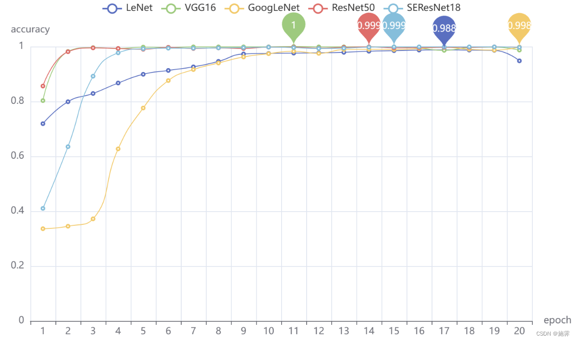
在训练过程中,VGG16与ResNet50在训练准确率以及损失值的变化上都十分接近,并且均迅速收敛,但VGG16更早的获得了最佳的权重参数,因此VGG16在所考虑因素的范围内略胜一筹。


考虑在测试集上的预测效果,根据上图我们可以看到,五个网络模型在测试集上的准确率都很高,除LeNet神经网络以外,其余四个模型都达到了99%以上,彼此之间的差距很小,VGG16仍然以略微的优势获得第一。
综合以上考虑,最终得出的结论是,VGG16模型在本次项目研究中表现结果最优,其余几个模型排名顺序依次为SEResNet18、ResNet50、GoogLeNet、LeNet。
今天的分享就到这啦,晚安~


 1294
1294


 被折叠的 条评论
为什么被折叠?
被折叠的 条评论
为什么被折叠?
 到【灌水乐园】发言


