[Probability] Conditional probability (2)

EricWang1358

于 2024-01-25 11:34:38 发布

阅读量799

点赞数 22

分类专栏： STA 文章标签： Probability

本文链接：https://blog.csdn.net/m0_74331272/article/details/135838608

版权

STA 专栏收录该内容

18 篇文章 0 订阅

订阅专栏

A new observation that is consistent with an existing belief could make us more sure of that belief, while a surprising observation could throw that belief into question.

Conditional probability is the concept that addresses this fundamental question: how should we update our beliefs in light of the evidence we observe?

2.1 The importance of thinking conditionally

In fact, a useful perspective is that all probabilities are conditional; whether or not it’s written explicitly, there is always background knowledge (or assumptions) built into every probability.

Definition 2.2.1

(Conditional probability). If A and B are events with P(B) > 0, then the conditional probability of A given B, denoted by P(A|B), is defined as $P(A|B)= \frac{P(A\cap B)}{P(B)}$

We call P(A) the prior probability of A and P(A|B) the posterior probability of A (“prior” means before updating based on the evidence, and “posterior” means after updating based on the evidence)

P(A|B) is the probability of A given the evidence B, not the probability of some entity called A|B. As discussed, there is no such event as A|B.

For any event A, P(A|A) = P(A ∩ A)/P(A) = 1.

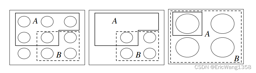
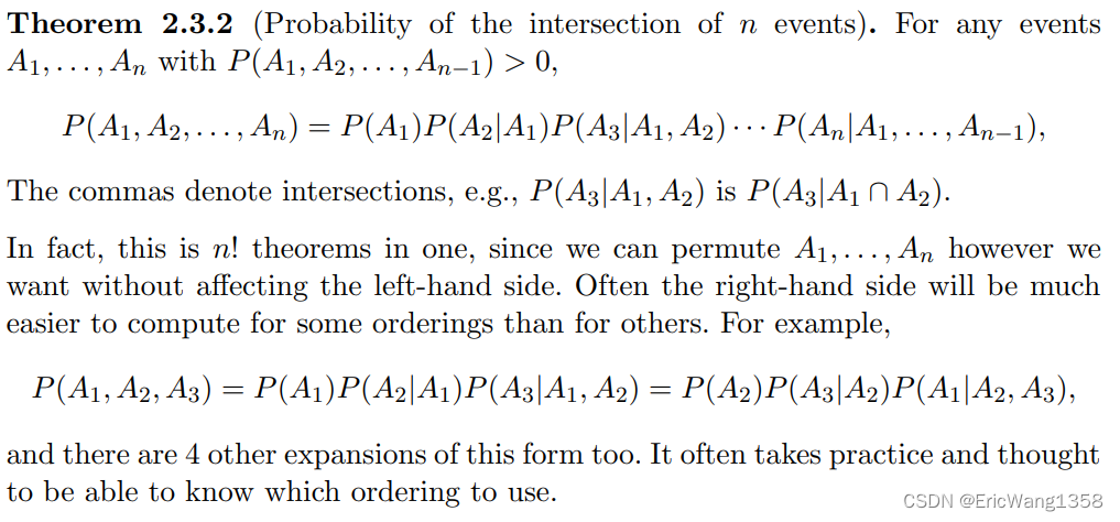
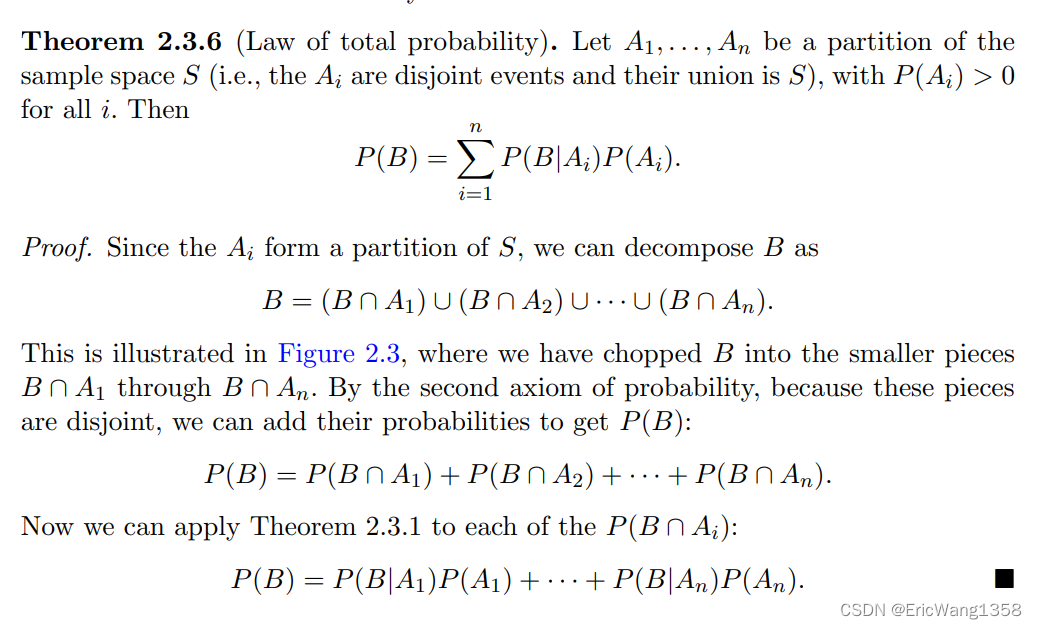
Intuition 2.2 (Pebble World).

Consider a finite sample space, with the outcomes visualized as pebbles with total mass 1. Since A is an event, it is a set of pebbles, and likewise for B. Figure 2.1(a) shows an example.

Intuition 2.2 (Frequentist interpretation).

Recall that the frequentist interpretation of probability is based on relative frequency over a large number of repeated trials. Imagine repeating our experiment many times, generating a long list of observed outcomes. The conditional probability of A given B can then be thought of in a natural way: it is the fraction of times that A occurs, restricting attention to the trials where B occurs

(Two children Problem)

[Probability] Conditional Probability-CSDN博客

2.3 Bayes’ rule and the law of total probability

Theorem 2.3.1 (Probability of the intersection of two events).

For any events A and B with positive probabilities, P(A ∩ B) = P(B)P(A|B) = P(A)P(B|A).

Theorem 2.3.2 (Probability of the intersection of n events).

Theorem 2.3.3 (Bayes’ rule).

$P(A|B) =\frac{P(B|A)P(A)}{P(B)}$

Another way to write Bayes’ rule is in terms of odds(赔率） rather than probability

Definition 2.3.4 (Odds).

The odds of an event A are $odds(A) = \frac{P(A)}{P(A^c)}$

For example, if P(A) = 2/3, we say the odds in favor of A are 2 to 1. (This is sometimes written as 2 : 1, and is sometimes stated as 1 to 2 odds against A; care is needed since some sources do not explicitly state whether they are referring to odds in favor or odds against an event.) Of course we can also convert from odds back to probability: $P(A) = \frac{odds(A)}{(1 + odds(A))}$

Theorem 2.3.5 (Odds form of Bayes’ rule).

For any events A and B with positive probabilities, the odds of A after conditioning on B are $\frac{P(A|B)}{P(A^c|B)}= (\frac{P(B|A)}{P(B|A^c)})\frac{P(A)}{P(A^c)}$

(from $\frac{P(A|B)P(B)}{P(A^c|B)P(B)}= \frac{P(B|A)}{P(B|A^c)}\frac{P(A)}{P(A^c)}$ )

In words, this says that the posterior odds P(A|B)/P(Ac|B) are equal to the prior odds P(A)/P(Ac ) times the factor P(B|A)/P(B|Ac ), which is known in statistics as the likelihood ratio.

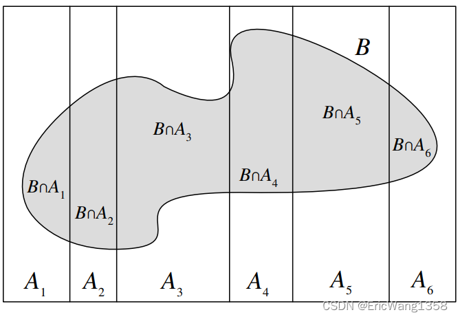
Theorem 2.3.6 (Law of total probability)

The law of total probability (LOTP) relates conditional probability to unconditional probability. It is essential for fulfilling the promise that conditional probability can be used to decompose complicated probability problems into simpler pieces, and it is often used in tandem with(与……协同；与……配合) Bayes’ rule.

A well-chosen partition will reduce a complicated problem into simpler pieces, whereas a poorly chosen partition will only exacerbate our problems, requiring us to calculate n difficult probabilities instead of just one!

(Random coin)

You have one fair coin, and one biased coin which lands Heads with probability 3/4. You pick one of the coins at random and flip it three times. It lands Heads all three times. Given this information, what is the probability that the coin you picked is the fair one?

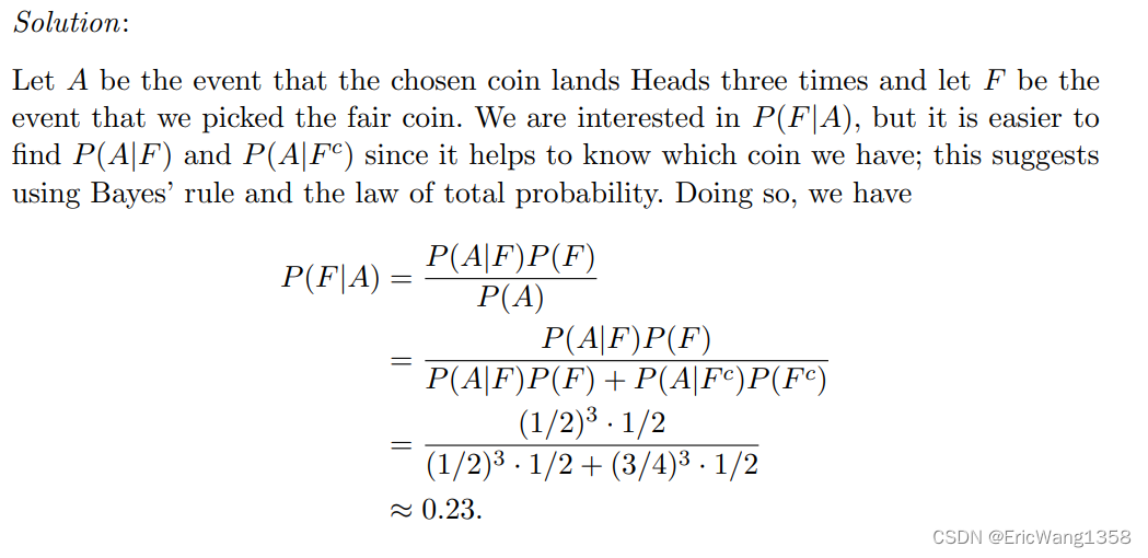
The key is how to compute the P(A) using the LOTP.

h 2.3.8 (Prior vs. posterior).

It would not be correct in the calculation in the above example to say after the first step, “P(A) = 1 because we know A happened.” It is true that P(A|A) = 1, but P(A) is the prior probability of A and P(F) is the prior probability of F—both are the probabilities before we observe any data in the 56 Introduction to Probability experiment. These must not be confused with posterior probabilities conditional on the evidence A.

Example 2.3.9 (Testing for a rare disease)

Most people find it surprising to learn that the conditional probability of having the disease given a positive test result is only 16%, even though the test is 95% accurate (see Gigerenzer and Hoffrage [13]). The key to understanding this surprisingly low posterior probability of having the disease is to realize that there are two factors at play: the evidence from the test, and our prior information about the prevalence of the disease.