[Prob] C4

Definition 4.1.1 (Expectation of a discrete r.v.).

Proposition 4.1.2. If X and Y are discrete r.v.s with the same distribution, then E(X) = E(Y ) (if either side exists)

h 4.1.3 (Replacing an r.v. by its expectation).A common mistake is to replace an r.v. by its expectation without justification,

 4.2 Linearity of expectation

Theorem 4.2.1 (Linearity of expectation).

Example 4.2.2 (Binomial expectation)

Example 4.2.3 (Hypergeometric expectation)

Proposition 4.2.4 (Monotonicity of expectation).

4.3 Geometric and Negative Binomial

Story 4.3.1 (Geometric distribution). until a success occurs

Theorem 4.3.2 (Geometric PMF).

Theorem 4.3.3 (Geometric CDF)

h 4.3.4 (Conventions for the Geometric).

In this book, the Geometric distribution excludes the success, and the First Success distribution includes the success.

Definition 4.3.5 (First Success distribution).

Example 4.3.6 (Geometric expectation)

Example 4.3.7 (First Success expectation).

The Negative Binomial distribution generalizes the Geometric distribution: instead of waiting for just one success, we can wait for any predetermined number r of successes

Story 4.3.8 (Negative Binomial distribution).

Theorem 4.3.9 (Negative Binomial PMF)

Theorem 4.3.10. Let X ∼ NBin(r, p), viewed as the number of failures before the rth success in a sequence of independent Bernoulli trials with success probability p. Then we can write X = X1 + · · · + Xr where the Xi are i.i.d. Geom(p).

Proof. Let X1 be the number of failures until the first success

Example 4.3.11 (Negative Binomial expectation).

Example 4.3.12 (Coupon collector).

4.3.13 (Expectation of a nonlinear function of an r.v.)

Example 4.3.14 (St. Petersburg paradox)

4.4 Indicator r.v.s and the fundamental bridge

Theorem 4.4.1 (Indicator r.v. properties）

IA∩B = IAIB.

IA∪B = IA + IB − IAIB

Theorem 4.4.2 (Fundamental bridge between probability and expectation)

IA ∼ Bern(p)

Example 4.4.3 (Boole, Bonferroni, and inclusion-exclusion).

Boole’s inequality or Bonferroni’s inequality

Theorem 4.4.1. For general n, we can use properties of indicator r.v.s as follows:

 Example 4.4.4 (Matching continued)

Example 4.4.5 (Distinct birthdays, birthday matches)

Example 4.4.6 (Putnam problem)

Example 4.4.7 (Negative Hypergeometric)

Finding the expected value of a Negative Hypergeometric

Theorem 4.4.8 (Expectation via survival function)

Example 4.4.9 (Geometric expectation redux)

 Theorem 4.5.1 (LOTUS)

4.6 Variance

Definition 4.6.1 (Variance and standard deviation)

Theorem 4.6.2.

If X and Y are independent, then Var(X + Y ) = Var(X) + Var(Y )

h 4.6.3 (Variance is not linear).

Example 4.6.4 (Geometric and Negative Binomial variance).

Example 4.6.5 (Binomial variance)

 

Definition 4.7.1 (Poisson distribution)

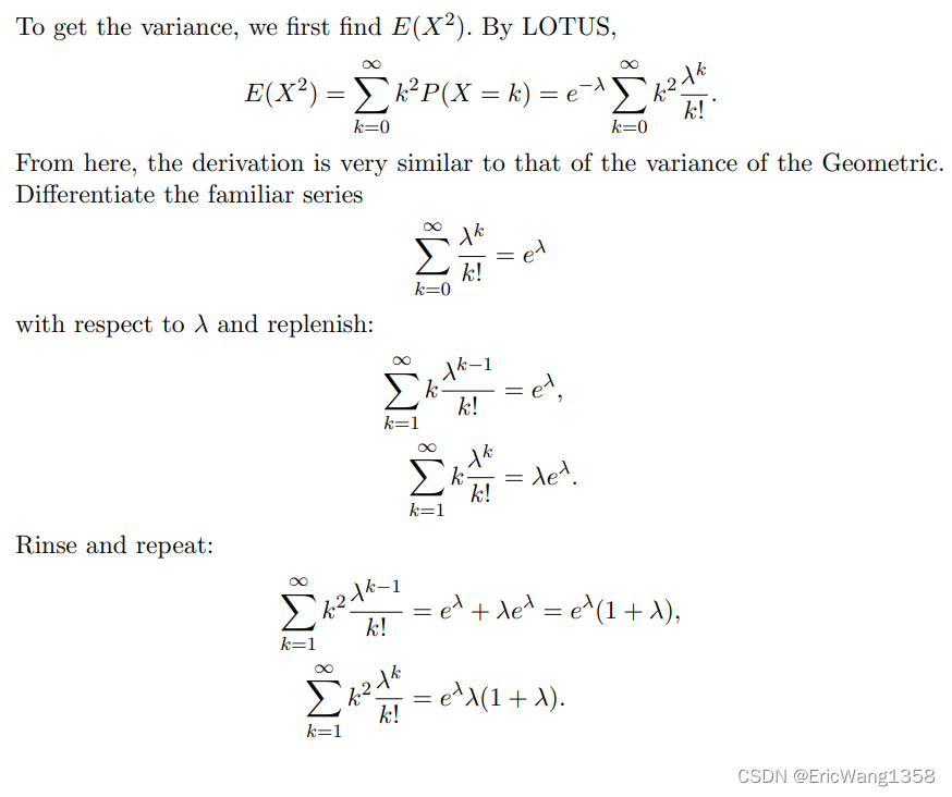
Example 4.7.2 (Poisson expectation and variance).

Approximation 4.7.3 (Poisson paradigm)

Example 4.7.4 (Balls in boxes).

Example 4.7.5 (Birthday problem continued).

Example 4.7.6 (Near-birthday problem).

Example 4.7.7 (Birth-minute and birth-hour).

4.8 Connections between Poisson and Binomial

Theorem 4.8.1 (Sum of independent Poissons)

Theorem 4.8.2 (Poisson given a sum of Poissons).

which is the Bin(n, λ1/(λ1 + λ2)) PMF, as desired.

Theorem 4.8.3 (Poisson approximation to Binomial).

Example 4.8.4 (Visitors to a website)