机器学习笔记(四)——支持向量机SVM

无情码手

已于 2022-04-30 21:21:19 修改

阅读量939

点赞数

分类专栏：机器学习笔记文章标签： python 机器学习

于 2022-04-30 21:13:44 首次发布

本文链接：https://blog.csdn.net/mars1533/article/details/124518804

版权

机器学习笔记专栏收录该内容

5 篇文章 0 订阅

订阅专栏

支持向量机SVM

逻辑回归

$h_{\theta}(x)=\frac{1}{1+e^{-\theta^{T} x}} \tag{1}$

$\text{If} \quad y=1, we \,\,\, want \,\,\, h_{\theta}(x) \approx 1, \quad \theta^{T} x \gg 0\\ \text{If} \quad y=0, we \,\,\, want \,\,\, h_{\theta}(x) \approx 0, \quad \theta^{T} x \ll 0 \tag{2}$

代价函数：
$\begin{aligned} \text{Cost} = &-\left(y \log h_{\theta}(x)+(1-y) \log \left(1-h_{\theta}(x)\right)\right)\\ =&-y \log \frac{1}{1+e^{-\theta^{T} x}}-(1-y) \log \left(1-\frac{1}{1+e^{-\theta^{T} x}}\right) \end{aligned} \tag{3}$

改进代价函数

SVM的代价函数是在逻辑回归的代价函数上进行改进，将 $(3)$ 式中的 $-\log h_{\theta}(x)$ 替换为 $\text{Cost}_1(x)$ ， $-\log \left(1-h_{\theta}(x)\right)$ 替换为 $\text{Cost}_0(x)$ 。下面两图是对 $\text{Cost}_1(x)$ 和 $\text{Cost}_0(x)$ 的介绍（红线部分代表 $\text{Cost}$ 函数）。

最终，SVM的代价函数修改为如下格式：
$\min _{\theta} C \sum_{i=1}^{m}\left[y^{(i)} \operatorname{cost}_{1}\left(\theta^{T} x^{(i)}\right)+\left(1-y^{(i)}\right) \operatorname{cost}_{0}\left(\theta^{T} x^{(i)}\right)\right]+\frac{1}{2} \sum_{i=1}^{n} \theta_{j}^{2} \tag{4}$
SVM代价函数共修改三处：

把逻辑回归里的两处函数改为 $\text{cost}_1$ 和 $\text{cost}_0$ ;
去掉了最前方的 $\frac{1}{m}$ （并不影响最优化），并且给第一项添加权重系数C，控制其权值;
去掉了正则项处的权重系数，由C控制相对权重。

SVM最终的输出有别于逻辑回归输出的概率。最小化代价函数获得参数 $\theta$ 时，支持向量机所做的是直接预测y值等于1还是等于0。
$h_{\theta}(x) \begin{cases}1 & \text { if } \theta^{T} x \geqslant 0 \\ 0 & \text { othervire }\end{cases} \tag{5}$

大间距分类器

下图是SVM的代价函数，左边是 $\text{Cost}_1(\theta^Tx)$ ，用于正样本，右边是 $\text{Cost}_0(\theta^Tx)$ ，用于负样本。最小化代价函数的条件是：当 $\theta^Tx \geq 1$ 时， $\text{Cost}_1(\theta^Tx)$ 才等于0。对于逻辑回归来说，当 $y = 0$ 时，希望 $\theta^Tx \leq 0$ ，当 $y = 1$ 时，希望 $\theta^Tx \geq 0$ 。换句话说，SVM的要求更高，相当于SVM中嵌入了安全的间距因子。

对于式 $(4)$ 来说，如果 $C$ 非常大，则最小化代价函数的时候，会希望找到使得第一项为0的最优解。因此可以等价为在代价项第一项为0情形下的优化问题。等价于下式。
$\min C \times 0+\frac{1}{2} \sum_{i=1}^{n} \theta_{i}^{2}\\ s.t. \theta^{T} x^{(i)} \geqslant 1 \quad if \,\,\, y^{(i)}=1,\\ \quad \,\,\,\theta^{T} x^{(i)} \leqslant-1 \quad if \,\,\, y^{(i)}=0.\tag{6}$
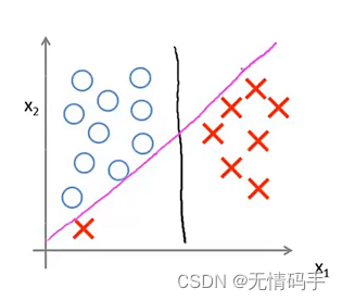
SVM会训练得到间距最大的黑色分界线，而并非下图中其他颜色的分界线。也就是说SVM鲁棒性较高，它用最大间距来分离样本。

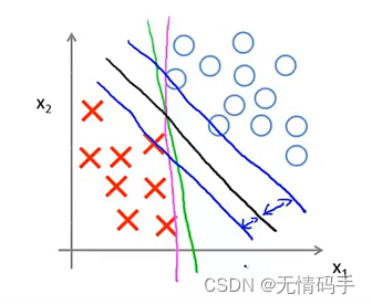
当 $C$ 设置较x小时，分界线为黑色（因为第一项没有占非常重要的地位，允许分错），但它的间距较大。当 $C$ 设置较大（第一项占据地位较大），分界线为由黑色变为紫色，间距变小。

大间距分类器的原因

要搞清楚这个问题，首先需要明白向量内积的另一种形式。
$\begin{aligned} \theta^{T} x^{(i)} &= \theta_{1} x_{1}^{(i)}+\theta_{2} x_{2}^{(i)}\\ &=p^{(i)}\|\theta\| \end{aligned} \tag{7}$
其中， $p^i$ 表示 $\theta$ 在 $x^i$ 上的投影，它有正有负。两向量夹角 $KaTeX parse error: Undefined control sequence: \textless at position 1: \̲t̲e̲x̲t̲l̲e̲s̲s̲ ̲90°$ 时， $p^i$ 为正，两向量夹角 $KaTeX parse error: Undefined control sequence: \textgreater at position 1: \̲t̲e̲x̲t̲g̲r̲e̲a̲t̲e̲r̲ ̲90°$ 时， $p^i$ 为负。
$\begin{aligned} &\min _{\theta} \frac{1}{2} \sum_{j=1}^{n} \theta_{j}^{2}\\ &\text { s.t. } p^{(i)} \cdot\|\theta\| \geq 1 \quad \text { if } y^{(i)}=1\\ &\quad \,\,\,\,\, p^{(i)} \cdot\|\theta\| \leq-1 \quad \text { if } y^{(i)}=1 \end{aligned} \tag{8}$
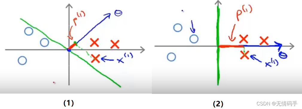
对于下图的两种情况来说，下图(1)中所示的 $p$ 很小，因为有 $p^{(i)} \cdot\|\theta\| \geq 1$ 和 $p^{(i)} \cdot\|\theta\| \leq -1$ 的约束，他会试图增大 $\|\theta\|$ ，显然这不符合我们的优化目标。换句话说，为达到我们的优化目标让 $\|\theta\|$ 尽可能小，SVM会选择较大的 $p^i$ 也就是下图(2)中所示的较大间距的决策边界。

提示：

$\theta_0=0$ 表示决策边界过原点， $\theta_0\,\, !=0$ 表示决策边界不过原点；
$\theta$ 与决策边界为垂直关系。因为边界公式为 $\theta^{T} x=\theta_{1} x_{1}+\theta_{2} x_{2}=0$ ，斜率为 $\frac{-\theta_1}{\theta_2}$ ， $\theta$ 为 $[\theta_1,\theta_2]^T$ ，斜率为 $\frac{\theta_2}{\theta_1}$ ，因此他们相互垂直。

核函数

核函数也可以称作similarity function，它描述了训练点和标记点之间的相似度(距离)。SVM可以定义标记点和核函数去构造一组新的特征 $f$ 代替原特征 $x$ 去进行模型的训练。一般来说，有多少训练点就有多少标记点。这里我们代表性地介绍一下高斯核函数。
$f^{(i)} = \left( \begin{array}{c} f_{1}^{(i)} \\ \vdots \\ f_{m}^{(i)} \end{array} \right)\\ f_{j}^{(i)}=\exp \left(-\frac{\left\|x^{(i)}-l^{{(j)}}\right\|^{2}}{2 \sigma^{2}}\right) \tag{9}$
其中， $f^{(i)}$ 是由高斯核函数和标记点构造出的新的特征，代表第 $i$ 个点与其他标记点间的相似度。 $f_j^{(i)}$ 代表原 $x^{(i)}$ 与第 $j$ 个标记点 $l^{(j)}$ 的相似度。也就是说，原来的特征 $x$ 被替换成了新的特征 $f$ ，它的格式由 $(m, n)$ 转变为了 $(m, m)$ 。此处 $\sigma$ 越小，函数下降越剧烈，计算相似度（距离）敏感度越高。 $\sigma$ 越大，函数下降越平缓，计算相似度（距离）敏感度越低。

最终，SVM的假设被修改为：给定 $x$ ，计算新特征 $f$ ，当 $\theta^Tf\geq0$ 时，预测 $y = 1$ ，否则反之。相应地，代价函数修改为如下公式。
$\min C \sum_{i=1}^{m}\left[y^{(i)} \operatorname{cost}_{1}\left(\theta^{T} f^{(i)}\right)+\left(1-y^{(i)}\right) \operatorname{cost}_{0}\left(\theta^{T} f^{(i)}\right)\right]+\frac{1}{2} \sum_{j=1}^{n=m} \theta_{j}^{2} \tag{10}$
需要注意的是，在计算 $\sum_{j=1}^{n=m} \theta_{j}^{2}=\theta^{T} \theta$ 时，为简化计算提高计算效率，用 $\theta^TM\theta$ 来代替。

另外，SVM也支持不使用核函数，也就是直接使用原来的特征 $x (m, n)$ 进行计算，代价函数也就是 $(4)$ 式，预测准则如下。
$\text { predict "y=1" \,\, if } \,\theta^{T} x \geqslant 0 \quad \left(\theta_{0}+\theta_{1} x_{1}+\cdots+\theta_{n} x_{n} \geqslant 0 \right) \tag{11}$

总结

SVM参数 $\sigma$ 和 $C$ 的影响

$1/\lambda$ ；
$C$ 较大时（ $\lambda$ ）较小，可能会导致过拟合，高方差；
$C$ 较小时（ $\lambda$ ）较大，可能会导致欠拟合，高偏差；
$\sigma$ 较大时，可能会导致低方差，高偏差；
$\sigma$ 较小时，可能会导致高方差，低偏差。

使用准则

n为特征数，m为训练样本数。

如果相较于m而言，n要大许多，即训练集数据量不够支持训练一个复杂的非线性模型，我们选用逻辑回归模型或者不带核函数的支持向量机。
如果n较小，而且m大小中等，例如n在1-1000之间，而m在10-10000之间，使用高斯核函数的支持向量机。
如果n较小，而m较大，例如n在1-1000之间，而m大于50000，则使用支持向量机会非常慢，解决方案是创造、增加更多的特征，然后使用逻辑回归或不带核函数的支持向量机。

代码

使用 DataFrame加载数据

raw_data = loadmat('data/ex6data1.mat')
# print(raw_data)
data = pd.DataFrame(raw_data['X'], columns=['X1', 'X2'])
data['y'] = raw_data['y']

# 把data['y']是1的data拿出来放在positive里
# 把data['y']是0的data拿出来放在negative里

positive = data[data['y'].isin([1])]
negative = data[data['y'].isin([0])]

绘制散点图

# figsize 设置图形的大小，a 为图形的宽， b 为图形的高
fig, ax = plt.subplots(figsize=(12,8))
# s 标记的大小
ax.scatter(positive['X1'], positive['X2'], s=50, marker='x', label='Positive')
ax.scatter(negative['X1'], negative['X2'], s=50, marker='o', label='Negative')
ax.legend()
plt.show()

不使用核函数的SVM（sklearn.svm.LinearSVC）

mat = sio.loadmat('./data/ex6data1.mat')
# 从mat里提取数值出来变成DataFrame
data = pd.DataFrame(mat.get('X'), columns=['X1', 'X2'])
# 增加新的一列'y'
data['y'] = mat.get('y')
#head()根据位置返回对象的前n行。如果你的对象中包含正确的数据类型, 则对于快速测试很有用。
#此方法用于返回数据帧或序列的前n行(默认值为5)。
print(data.head())

#可视化数据
fig, ax = plt.subplots(figsize=(8,6))
#c 颜色区分 ->按y来区分颜色
ax.scatter(data['X1'], data['X2'], s=50, c=data['y'], cmap='Reds')
ax.set_title('Raw data')
ax.set_xlabel('X1')
ax.set_ylabel('X2')
plt.show()

#try  C = 1
#loss : string, ‘hinge’ or ‘squared_hinge’ (default=’squared_hinge’)
#指定损失函数。 “hinge”是标准的SVM损失（例如由SVC类使用），而“squared_hinge”是hinge损失的平方。
svc1 = sklearn.svm.LinearSVC(C=1, loss='hinge')
svc1.fit(data[['X1', 'X2']], data['y'])
print(svc1.score(data[['X1', 'X2']], data['y']))

#try  C = 100
svc100 = sklearn.svm.LinearSVC(C=100, loss='hinge')
svc100.fit(data[['X1', 'X2']], data['y'])
print(svc100.score(data[['X1', 'X2']], data['y']))

使用高斯核函数的SVM（sklearn.svm.SVC）

# kernek function
def gaussian_kernel(x1, x2, sigma):
    return np.exp(- np.power(x1 - x2, 2).sum() / (2 * (sigma ** 2)))

#load data
mat = sio.loadmat('./data/ex6data2.mat')
print(mat.keys())
data = pd.DataFrame(mat.get('X'), columns=['X1', 'X2'])
data['y'] = mat.get('y')

#可视化数据
#palette 调色板
sns.set(context="notebook", style="white", palette=sns.diverging_palette(240, 10, n=2))
# data 参数是DataFrame
# ‘X1’ 'X2'表示横纵坐标名称
# hue 表示区分的名称 这里是y 用于分类
# fit_reg:(可选)此参数接受bool值。如果为True，则估计并绘制与x和y变量相关的回归模型。
# height:(可选)此参数是每个构面的高度(以英寸为单位)。
sns.lmplot('X1', 'X2', hue='y', data=data,
           height=5,
           fit_reg=False,
           scatter_kws={"s": 10}
          )
plt.show()

# try built-in Gaussian Kernel of sklearn
# radial basis function（Gaussian）kernel，简称 RBF kernel
svc = svm.SVC(C=100, kernel='rbf', gamma=10, probability=True)
print(svc)
svc.fit(data[['X1', 'X2']], data['y'])
print(svc.score(data[['X1', 'X2']], data['y']))

置信水平计算

# 查看每个类别预测的置信水平
data['SVM 1 Confidence'] = svc.decision_function(data[['X1', 'X2']])

fig, ax = plt.subplots(figsize=(12,8))
ax.scatter(data['X1'], data['X2'], s=50, c=data['SVM 1 Confidence'], cmap='seismic')
ax.set_title('SVM (C=1) Decision Confidence')
#plt.show()

data['SVM 2 Confidence'] = svc2.decision_function(data[['X1', 'X2']])

fig, ax = plt.subplots(figsize=(12,8))
ax.scatter(data['X1'], data['X2'], s=50, c=data['SVM 2 Confidence'], cmap='seismic')
ax.set_title('SVM (C=100) Decision Confidence')
plt.show()

#从图中可以看出 C = 1 的分类效果更好，置信度更高

最佳 $C$ 和 $\sigma$ 寻找

#找最佳的 C 和 \sigma
raw_data = loadmat('data/ex6data3.mat')

X = raw_data['X']
Xval = raw_data['Xval']
y = raw_data['y'].ravel()
yval = raw_data['yval'].ravel()

C_values = [0.01, 0.03, 0.1, 0.3, 1, 3, 10, 30, 100]
gamma_values = [0.01, 0.03, 0.1, 0.3, 1, 3, 10, 30, 100]

best_score = 0
best_params = {'C': None, 'gamma': None}

for C in C_values:
    for gamma in gamma_values:
        svc = svm.SVC(C=C, gamma=gamma)
        svc.fit(X, y)
        score = svc.score(Xval, yval)

        if score > best_score:
            best_score = score
            best_params['C'] = C
            best_params['gamma'] = gamma

print(best_score, best_params)

使用SVM构建垃圾邮件分类器

spam_train = loadmat('data/spamTrain.mat')
spam_test = loadmat('data/spamTest.mat')

X = spam_train['X']
Xtest = spam_test['Xtest']
y = spam_train['y'].ravel()
ytest = spam_test['ytest'].ravel()

svc = svm.SVC()
svc.fit(X, y)
print('Training accuracy = {0}%'.format(np.round(svc.score(X, y) * 100, 2)))
print('Test accuracy = {0}%'.format(np.round(svc.score(Xtest, ytest) * 100, 2)))

无情码手

关注

0
点赞
踩
0

收藏

觉得还不错? 一键收藏
0
评论
机器学习笔记(四)——支持向量机SVM

支持向量机SVM逻辑回归hθ(x)=11+e−θTx(1)h_{\theta}(x)=\frac{1}{1+e^{-\theta^{T} x}} \tag{1}hθ(x)=1+e−θTx1(1)Ify=1,we want hθ(x)≈1,θTx≫0Ify=0,we want hθ(x)≈0,θTx≪0(2)\text{If} \quad y=1, we \,\,\, want \,\,\, h_{\theta}(x) \approx 1, \quad \theta^{T} x
复制链接

扫一扫