


 本文探讨了Kaggle婚姻与离婚数据集,通过Levenberg-Marquardt和PSO优化算法,对比神经网络(NN)与普通回归方法预测离婚概率。使用Matlab实现,展示了深度学习在理解婚姻特征与离婚风险之间的复杂关系上的优势。
1 内容介绍
(婚姻和离婚数据))
Marriage and Divorce Dataset | Kaggle 数据集信息:
此数据包含 31 列 (100x31)。前 30 列是特征(输入),即年龄差距、教育程度、经济相似性、社会相似性、文化相似性、社会差距、共同兴趣、宗教相容性、前婚子女数量、结婚愿望、独立性、与父母的关系配偶家庭,交易,订婚时间,爱情,承诺,心理健康,生孩子的感觉,以前的交易,以前的婚姻,共同基因的比例,成瘾,忠诚度,身高比,良好的收入,自信,与非-婚前配偶、家庭确认配偶、家庭离婚1级开始与异性交往。第 31 列是离婚概率(目标)。
任何人都可以通过适当的确认/引用来使用这些数据。属性信息:该数据包含 30 个特征(输入)和一个目标。特点是:
-
年龄差距 2. 教育程度 3. 经济相似度 4. 社会相似度 5. 文化相似度 6. 社会差距 7. 共同利益 8. 宗教相容性 9. 前婚子女数量 10. 结婚意愿 11. 独立性 12. 与他人的关系配偶家庭 13.交易 14.订婚时间 15.爱情 16.承诺 17.心理健康 18.生孩子的感觉 19.以前的交易 20.以前的婚姻 21.共同基因的比例 22.成瘾 23.忠诚度 24.身高比例 25.良好的收入 26.自信心 27.婚前与非配偶的关系 28.家庭确认的配偶 29.一级家庭离婚 30.开始与异性交往 目标是离婚概率。
2 仿真代码
clear;
close all
Data=load('Marriage_Divorce_DB.mat');
Inputs=Data.Marriage_Divorce_DB(:,1:end-1);
Targets=Data.Marriage_Divorce_DB(:,end);
%% Learning
n = 9; % Neurons
%----------------------------------------
% 'trainlm' Levenberg-Marquardt
% 'trainbr' Bayesian Regularization (good)
% 'trainrp' Resilient Backpropagation
% 'traincgf' Fletcher-Powell Conjugate Gradient
% 'trainoss' One Step Secant (good)
% 'traingd' Gradient Descent
% Creating the NN ----------------------------
net = feedforwardnet(n,'trainoss');
%---------------------------------------------
% configure the neural network for this dataset
[net tr]= train(net,Inputs', Targets');
perf = perform(net,Inputs, Targets); % mse
% Current NN Weights and Bias
Weights_Bias = getwb(net);
% MSE Error for Current NN
Outputs=net(Inputs');
Outputs=Outputs';
% Final MSE Error and Correlation Coefficients (CC)
Err_MSE=mse(Targets,Outputs);
CC1= corrcoef(Targets,Outputs);
CC1= CC1(1,2);
%-----------------------------------------------------
%% Nature Inspired Regression
% Create Handle for Error
h = @(x) NMSE(x, net, Inputs', Targets');
sizenn=size(Inputs);sizenn=sizenn(1,1);
%-----------------------------------------
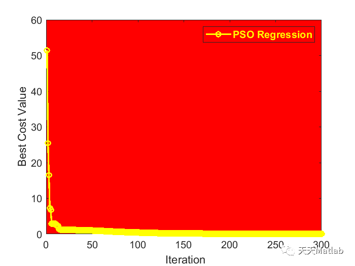
%% Please select BBO (bbo) or PSO (pso)
[x, cost] = pso(h, sizenn*n+n+n+1);
%-----------------------------------------
net = setwb(net, x');
% Optimized NN Weights and Bias
getwb(net);
% Error for Optimized NN
Outputs2=net(Inputs');
Outputs2=Outputs2';
% Final MSE Error and Correlation Coefficients (CC)
Err_MSE2=mse(Targets,Outputs2);
CC2= corrcoef(Targets,Outputs2);
CC2= CC2(1,2);
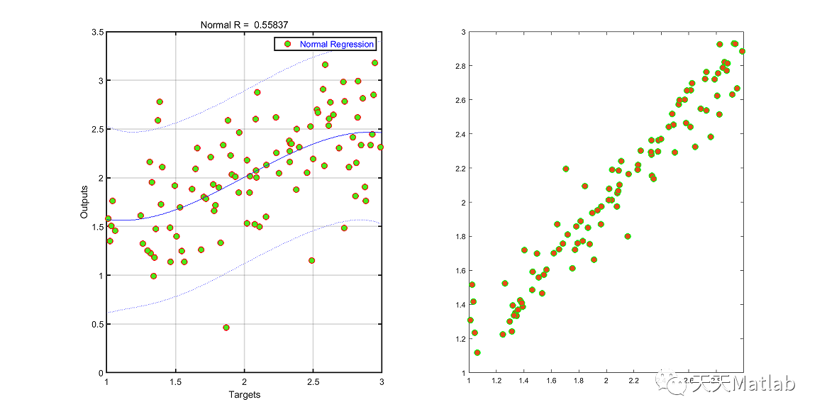
%% Plot Regression
figure('units','normalized','outerposition',[0 0 1 1])
% Normal
subplot(1,2,1)
[population2,gof] = fit(Targets,Outputs,'poly3');
plot(Targets,Outputs,'o',...
'LineWidth',1,...
'MarkerSize',8,...
'MarkerEdgeColor','r',...
'MarkerFaceColor',[0.3,0.9,0.1]);
title(['Normal R = ' num2str(1-gof.rmse)],['Normal MSE = ' num2str(Err_MSE)]);
hold on
plot(population2,'b-','predobs');
xlabel('Targets');ylabel('Outputs'); grid on;
ax = gca;
ax.FontSize = 12; ax.LineWidth=2;
legend({'Normal Regression'},'FontSize',12,'TextColor','blue');hold off
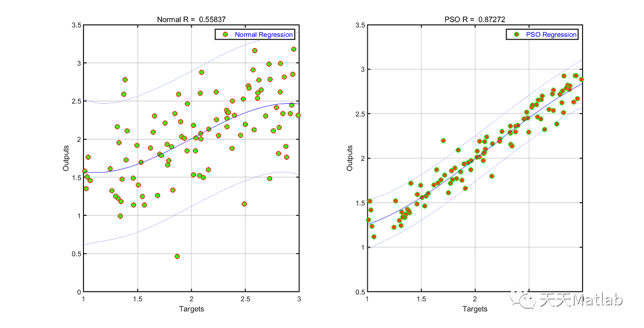
% PSO
subplot(1,2,2)
[population3,gof3] = fit(Targets,Outputs2,'poly3');
plot(Targets,Outputs2,'o',...
'LineWidth',1,...
'MarkerSize',8,...
'MarkerEdgeColor','g',...
'MarkerFaceColor',[0.9,0.3,0.1]);
title(['PSO R = ' num2str(1-gof3.rmse)],['PSO MSE = ' num2str(Err_MSE2)]);
hold on
plot(population3,'b-','predobs');
xlabel('Targets');ylabel('Outputs'); grid on;
ax = gca;
ax.FontSize = 12; ax.LineWidth=2;
legend({'PSO Regression'},'FontSize',12,'TextColor','blue');hold off
% Correlation Coefficients
fprintf('Normal Correlation Coefficients Is = %0.4f.\n',CC1);
fprintf('PSO Correlation Coefficients Is = %0.4f.\n',CC2);
3 运行结果
4 参考文献
[1] Zimmermann h.j. “fuzzy set theory and its applications”, 2nd edition,kluwer academic pub,(1991).
[2] Klir, G. J., & Folger, T .A., “Fuzzy sets,Uncertainty,and Information”,Prentice-Hall,(1988).
[3] Mosqueira-Rey, E., Moret-Bonillo, V., & Fernández-Leal, Á. (2008). “An expert system to achieve fuzzy
interpretations of validation data. Expert Systems with Applications”, 35(4), 2089–2106.
[4] Eiben, Agoston E., and James E. Smith. Introduction to evolutionary computing. Vol. 53. Heidelberg: springer, 2003.
[5] R. Storn and K. Price. Differential Evolution: A Simple and Efficient Adaptive Scheme for Global Optimization over Continuous Spaces. Technical Report TR-95-012, International Computer Science Institute, Berkeley, California,March 1995.
[6] R. Storn and K. Price. Differential Evolution - A Fast and Efficient Heuristic for Global Optimization over Continuous Spaces. Journal of Global Optimization, 11:341–359, 1997.
博主简介:擅长智能优化算法、神经网络预测、信号处理、元胞自动机、图像处理、路径规划、无人机等多种领域的Matlab仿真,相关matlab代码问题可私信交流。
部分理论引用网络文献,若有侵权联系博主删除。


 1205
1205

 被折叠的 条评论
为什么被折叠?
被折叠的 条评论
为什么被折叠?
 到【灌水乐园】发言


