Understanding Gated Recurrent Unit (GRU) in Deep Learning

Source

What is Gated Recurrent Unit(GRU) ?

GRU stands for Gated Recurrent Unit, which is a type of recurrent neural network (RNN) architecture that is similar to LSTM (Long Short-Term Memory).

Like LSTM, GRU is designed to model sequential data by allowing information to be selectively remembered or forgotten over time. However, GRU has a simpler architecture than LSTM, with fewer parameters, which can make it easier to train and more computationally efficient.

LSTM

https://blog.mlreview.com/understanding-lstm-and-its-diagrams-37e2f46f1714

Theoretically the naively connected neural network, so called recurrent neural network, can work. But in practice, it suffers from two problems: vanishing gradient and exploding gradient, which make it unusable.

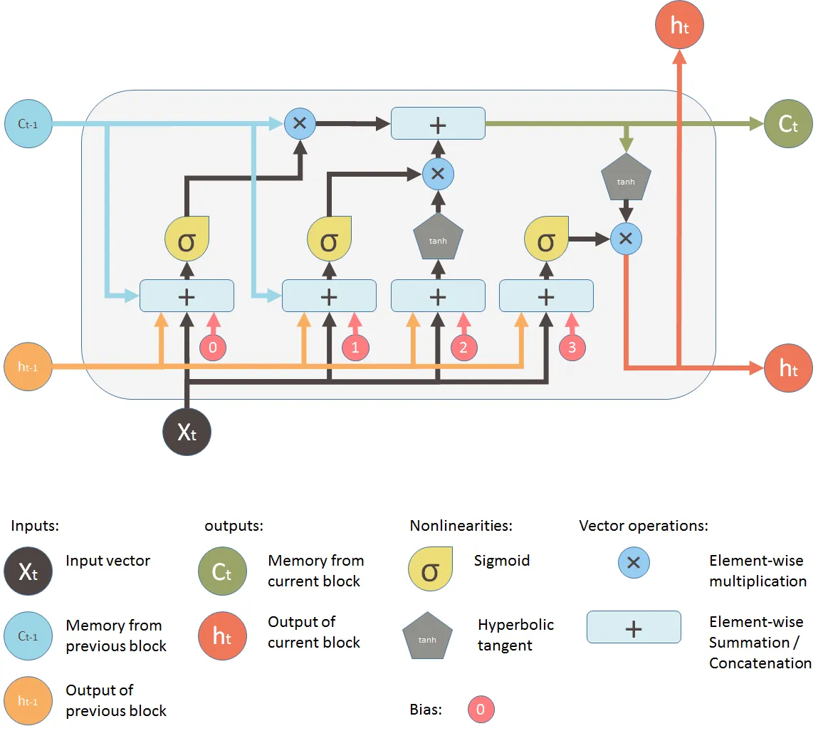
==> here is the classic pipeline-oriented unit diagram cell:

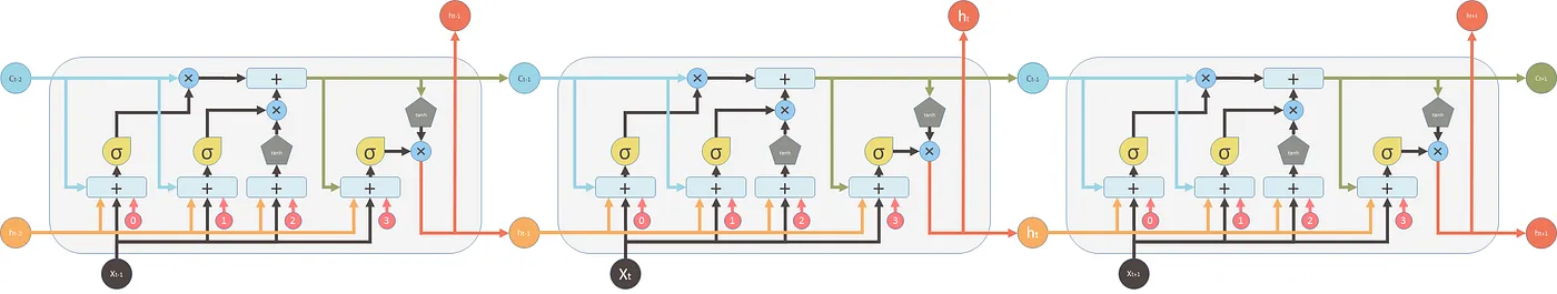
in tandem:

for a cell/gate-centered unit diagram:

 

(Based on Bard)

As you can see, the LSTM unit consists of four main components:

• Cell state: The cell state is a long-term memory that stores information over time. It is represented by a vector of values, and it is updated at each time step based on the input and the previous cell state.
• Forget gate (0): The forget gate decides what information to throw away from the cell state. It is a sigmoid function that takes the X_t, h_t-1, (C_t-1,) and outputs a value between 0 and 1. A value of 1 means to keep the information, and a value of 0 means to throw it away.
• Input gate (1): The input gate decides what new information to add to the cell state. It is a sigmoid function that takes the X_t, h_t-1, (C_t-1,) as input, and outputs a value between 0 and 1. A value of 1 means to add the new information, and a value of 0 means to ignore it.
• Output gate (3): The output gate decides what information to output from the LSTM unit. It is a sigmoid function that takes (X_t,) h_t-1, C_t as input, and outputs a value between 0 and 1. A value of 1 means to output the information, and a value of 0 means to not output it.

The LSTM unit also has two additional components:

• Input transform (2): The input transform is a tanh function that takes the input and the previous hidden state as input, and outputs a vector of values.
• Hidden state/Output transform (the other tanh): The hidden state transform is a tanh function that takes the current cell state as input, and outputs a vector of values.

==> the IO transforms are the key for LSTM to avoid gradient extrema, essentially we introduced tanh to remap IO, recall that tanh is:

centered at 0,

bounded between -1 and 1

differentiable

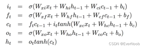
The LSTM unit works as follows:

The cell state is then updated using the following formula:

C_t = f_t * C_{t-1} + i_t * tanh(W_i[h_{t-1}, x_t])

where:

• C_t is the cell state at time step t
• f_t is the forget gate value at time step t
• i_t is the input gate value at time step t
• W_i is the weight matrix for the input transform
• h_{t-1} is the hidden state at time step t-1
• x_t is the input at time step t

The hidden state is then updated using the following formula:

h_t = o_t * tanh(C_t)

where:

• h_t is the hidden state at time step t
• o_t is the output gate value at time step t

The output of the LSTM unit is the hidden state h_t.

The main difference between GRU and LSTM is the way they handle the memory cell state. In LSTM, the memory cell state is maintained separately from the hidden state and is updated using three gates: the input gate, output gate, and forget gate. In GRU, the memory cell state is replaced with a “candidate activation vector,” which is updated using two gates: the reset gate and update gate.

The reset gate determines how much of the previous hidden state to forget, while the update gate determines how much of the candidate activation vector to incorporate into the new hidden state.

Overall, GRU is a popular alternative to LSTM for modeling sequential data, especially in cases where computational resources are limited or where a simpler architecture is desired.

How GRU Works?

Like other recurrent neural network architectures, GRU processes sequential data one element at a time, updating its hidden state based on the current input and the previous hidden state. At each time step, the GRU computes a “candidate activation vector” that combines information from the input and the previous hidden state. This candidate vector is then used to update the hidden state for the next time step.

The candidate activation vector is computed using two gates: the reset gate and the update gate. The reset gate determines how much of the previous hidden state to forget, while the update gate determines how much of the candidate activation vector to incorporate into the new hidden state.

Here’s the math behind the GRU architecture:

1. The reset gate r and update gate z are computed using the current input x and the previous hidden state h_t-1

r_t = sigmoid(W_r * [h_t-1, x_t])
z_t = sigmoid(W_z * [h_t-1, x_t])

where W_r and W_z are weight matrices that are learned during training.

2. The candidate activation vector h_t~ is computed using the current input x and a modified version of the previous hidden state (r_t) that is "reset" by the reset gate:

h_t~ = tanh(W_h * [r_t * h_t-1, x_t])

where W_h is another weight matrix.

3. The new hidden state h_t is computed by combining the candidate activation vector with the previous hidden state, weighted by the update gate:

h_t = (1 - z_t) * h_t-1 + z_t * h_t~

Overall, the reset gate determines how much of the previous hidden state to remember or forget, while the update gate determines how much of the candidate activation vector to incorporate into the new hidden state. The result is a compact architecture that is able to selectively update its hidden state based on the input and previous hidden state, without the need for a separate memory cell state like in LSTM.

GRU Architecture

The GRU architecture consists of the following components:

1. Input layer: The input layer takes in sequential data, such as a sequence of words or a time series of values, and feeds it into the GRU.
2. Hidden layer: The hidden layer is where the recurrent computation occurs. At each time step, the hidden state is updated based on the current input and the previous hidden state. The hidden state is a vector of numbers that represents the network’s “memory” of the previous inputs.
3. Reset gate: The reset gate determines how much of the previous hidden state to forget. It takes as input the previous hidden state and the current input, and produces a vector of numbers between 0 and 1 that controls the degree to which the previous hidden state is “reset” at the current time step.
4. Update gate: The update gate determines how much of the candidate activation vector to incorporate into the new hidden state. It takes as input the previous hidden state and the current input, and produces a vector of numbers between 0 and 1 that controls the degree to which the candidate activation vector is incorporated into the new hidden state.
5. Candidate activation vector: The candidate activation vector is a modified version of the previous hidden state that is “reset” by the reset gate and combined with the current input. It is computed using a tanh activation function that squashes its output between -1 and 1.
6. Output layer: The output layer takes the final hidden state as input and produces the network’s output. This could be a single number, a sequence of numbers, or a probability distribution over classes, depending on the task at hand.

Pros and Cons of GRU

Like any machine learning model, Gated Recurrent Unit (GRU) neural networks have both advantages and disadvantages. Here are some pros and cons of using GRU:

Pros:

• GRU networks are similar to Long Short-Term Memory (LSTM) networks, but with fewer parameters, making them computationally less expensive and faster to train.
• GRU networks can handle long-term dependencies in sequential data by selectively remembering and forgetting previous inputs.
• GRU networks have been shown to perform well on a variety of tasks, including natural language processing, speech recognition, and music generation.
• GRU networks can be used for both sequence-to-sequence and sequence classification tasks.

Cons:

• GRU networks may not perform as well as LSTMs on tasks that require modeling very long-term dependencies or complex sequential patterns.
• GRU networks may be more prone to overfitting than LSTMs, especially on smaller datasets.
• GRU networks require careful tuning of hyperparameters, such as the number of hidden units and learning rate, to achieve good performance.
• GRU networks may not be as interpretable as other machine learning models, since the gating mechanism can make it difficult to understand how the network is making predictions.

Overall, GRU networks are a powerful tool for modeling sequential data, especially in cases where computational resources are limited or where a simpler architecture is desired. However, like any machine learning model, they have their limitations and require careful consideration when choosing the appropriate model for a particular task.