AdaBoost 算法基础（二分类）

最新推荐文章于 2024-06-28 15:22:31 发布

ViolinLeeChan

最新推荐文章于 2024-06-28 15:22:31 发布

阅读量3.2k

点赞数

分类专栏：机器学习（Machine Learning）

本文链接：https://blog.csdn.net/mechleechan/article/details/87900068

版权

机器学习（Machine Learning）专栏收录该内容

5 篇文章 2 订阅

订阅专栏

所属知识点：Machine Learning：Boosting
归纳和总结机器学习技术的库：ViolinLee/ML_notes。该库主要内容是我的机器学习笔记，同时挑选和收集各类与机器学习技术相关的高质量资源，欢迎大家关注和Star！会一直更新下去。
微信公众号：“RoboticsCV”（微信号：ModernRobotics）。公众号专注机器人学，关注机器学习、计算机视觉等前沿技术在机器人领域中的应用。公众号将分享与机器人相关的重要知识和前沿技术，同时保证文章的质量，对总结和分享的各个技术，尽量做到在概念，项目，学习资源上都对大家有充分帮助。公众号刚注册，很快会运营，欢迎大家关注！

AdaBoost（Adaptive Boosting，自适应增强）属于提升方法（Boosting）的一种，由Yoav Freund和Robert Schapire提出。AdaBoost方法的自适应在于：前一个分类器分错的样本会被用来训练下一个分类器。AdaBoost 方法对于噪声数据和异常数据很敏感。但在一些问题中，AdaBoost 方法相对于大多数其它学习算法而言，不会很容易出现过拟合现象。

注意：AdaBoost 方法中使用的分类器可能很弱（比如出现很大错误率），但只要它的分类效果比随机好一点（比如两类问题分类错误率略小于0.5），就能够改善最终得到的模型。而错误率高于随机分类器的弱分类器也是有用的，因为在最终得到的多个分类器的线性组合中，可以给它们赋予负系数，同样也能提升分类效果。

1. Adaboost 原理
AdaBoost 方法是一种迭代算法，在每一轮中加入一个新的弱分类器，直到达到某个预定的足够小的错误率。每一个训练样本都被赋予一个权重，表明它被某个分类器选入训练集的概率。如果某个样本点已经被准确地分类，那么在构造下一个训练集中，它被选中的概率就被降低；相反，如果某个样本点没有被准确地分类，那么它的权重就得到提高。通过这样的方式，AdaBoost 方法能“聚焦于”那些较难分（更富信息）的样本上。

具体实现：
（1）初始化训练数据（每个样本）的权值分布：最初令每个样本的权重都相等。
（2）训练弱分类器：对于第k次迭代操作，我们就根据每个样本的权重来选取样本点，进而训练分类器 $C_{k}$ 。然后根据这个分类器，提高被它错误分类的样本的权重，并降低被正确分类的样本权重。然后，权重更新过的样本集被用于训练下一个分类器 $C_{k+1}$ 。整个训练过程如此迭代地进行下去。
（3）将各个训练得到的弱分类器组合成强分类器：各个弱分类器的训练过程结束后，分类误差率小的弱分类器的话语权较大，其在最终的分类函数中起着较大的决定作用，而分类误差率大的弱分类器的话语权较小，其在最终的分类函数中起着较小的决定作用。换言之，误差率低的弱分类器在最终分类器中占的比例较大，反之较小。

关键概念：
迭代算法；每个样本的权重；弱分类器的话语权（权重）；

2. Adaboost 优劣
优点
1) Adaboost 是一种高精度分类器
2) Adaboost 算法提供的是框架，因此可以使用各种方法构建子分类器
3) 当使用简单分类器时，计算出的结果是可以理解的。而且弱分类器构造极其简单
4) 简单，不需要做特征筛选
5) 不容易出现过拟合
缺点
1) 对噪声敏感，但这亦是大部分算法的缺点
2) 训练时间长
3) 执行效果依赖于弱分类器的选择

3. Adaboost 算法流程
迭代过程：

图解：

数学描述：
第一步：初始化训练数据的权值分布。

其中， $D_{1}$ 表示第一次迭代时每个样本的权值， $w_{11}$ 表示第一次迭代时第一个样本的权值， $N$ 为样本总数。

第二步：进行 M 次迭代。
a) 使用拥有权值分布 $D_{m}\left ( m=1,2,3,...,N \right )$ 的训练样本进行学习，得到弱分类器: $G_{m}\left ( x \right ): x\rightarrow \left \{ -1,1 \right \}$ 。
弱分类器的性能指标通过以下误差函数的值 $\epsilon _{m}$ 来衡量：
$\epsilon _{m}=\sum_{n=1}^{N}w_{mn}I\left ( y_{m}\left ( x_{n} \right ) \right \neq t_{n})$

b) 计算弱分类器 $G_{m}$ 的话语权 $\alpha _{m}$ （亦是权值），它表示 $G_{m}$ 在最终分类器中的重要程度。计算方法如下：

è¿éåå¾çæè¿°

随着 $e_{m}$ 减小， $\alpha _{m}$ 逐渐增大。该式表明，误差率小的分类器，在最终分类器中的重要程度大。

c) 更新训练样本的权值分布，用于下一轮迭代。被错误分类的样本权值增加；被正确分类的样本权值减小。计算方法如下：
$D_{m+1}=\left ( w_{m+1,1},w_{m+1,2},...,w_{m+1,i},...,w_{m+1,N} \right )$
$w_{m+1,i}=\frac{w_{mi}}{Z_{m}}e^{-\alpha _{m}y_{i}G_{m}\left ( x_{i} \right )}, i=1,2,...,N$
其中， $D_{m+1}$ 是用于下次迭代时样本的权值， $w_{m+1,1}$ 是下一次迭代时，第 $i$ 个样本的权值。 $y_{i}$ 代表第 $i$ 个样本对应的类别（1 或 -1）， $G_{m}\left ( x_{i} \right )$ 表示弱分类器对样本 $x_{i}$ 的分类（1 或 -1）。若分类正确，则 $y_{i}G_{m}\left ( x_{i} \right )$ 的值为1，反之为-1。其中 $Z_{m}$ 是归一化因子，计算方法如下：

第三步：组合弱分类器，获得强分类器
首先，对所有迭代过的分类器加权求和：

接着，将 sign 函数作用于求和结果，得到最终的强分类器 $G\left ( x \right )$ ：

sign 函数（符号函数，简称 sgn）：是一个逻辑函数，用以判断实数的正负号。其定义为：

$\operatorname{sgn} x=\left\{{\begin{matrix}-1&:&x<0\\0&:&x=0\\1&:&x>0\end{matrix}}\right.$

4. Adaboost 代码实现
4.1 Python 实现
借助 SKlearn 内置的数据集、基础分类器（决策树）、交叉验证函数，使用 Python 实现 Adaboost。以下为实现代码：
adaboost_implementation.ipynb (基于 python 2.7；scikit-learn v0.20.2)

import pandas as pd
import numpy as np
from sklearn.tree import DecisionTreeClassifier
from sklearn.model_selection import train_test_split
from sklearn.datasets import make_hastie_10_2
import matplotlib.pyplot as plt

""" HELPER FUNCTION: GET ERROR RATE ========================================="""
def get_error_rate(pred, Y):
    return sum(pred != Y) / float(len(Y))

""" HELPER FUNCTION: PRINT ERROR RATE ======================================="""
def print_error_rate(err):
    print 'Error rate: Training: %.4f - Test: %.4f' % err

""" HELPER FUNCTION: GENERIC CLASSIFIER ====================================="""
def generic_clf(Y_train, X_train, Y_test, X_test, clf):
    clf.fit(X_train,Y_train)
    pred_train = clf.predict(X_train)
    pred_test = clf.predict(X_test)
    return get_error_rate(pred_train, Y_train), \
           get_error_rate(pred_test, Y_test)
    
""" ADABOOST IMPLEMENTATION ================================================="""
def adaboost_clf(Y_train, X_train, Y_test, X_test, M, clf):
    n_train, n_test = len(X_train), len(X_test)
    # Initialize weights
    w = np.ones(n_train) / n_train
    pred_train, pred_test = [np.zeros(n_train), np.zeros(n_test)]
    
    for i in range(M):
        # Fit a classifier with the specific weights
        clf.fit(X_train, Y_train, sample_weight = w)
        pred_train_i = clf.predict(X_train)
        pred_test_i = clf.predict(X_test)
        # Indicator function
        miss = [int(x) for x in (pred_train_i != Y_train)]
        # Equivalent with 1/-1 to update weights
        miss2 = [x if x==1 else -1 for x in miss]
        # Error
        err_m = np.dot(w,miss) / sum(w)
        # Alpha
        alpha_m = 0.5 * np.log( (1 - err_m) / float(err_m))
        # New weights
        w = np.multiply(w, np.exp([float(x) * alpha_m for x in miss2]))
        # Add to prediction
        pred_train = [sum(x) for x in zip(pred_train, 
                                          [x * alpha_m for x in pred_train_i])]
        pred_test = [sum(x) for x in zip(pred_test, 
                                         [x * alpha_m for x in pred_test_i])]
    
    pred_train, pred_test = np.sign(pred_train), np.sign(pred_test)
    # Return error rate in train and test set
    return get_error_rate(pred_train, Y_train), \
           get_error_rate(pred_test, Y_test)

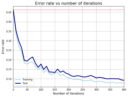
""" PLOT FUNCTION ==========================================================="""
def plot_error_rate(er_train, er_test):
    df_error = pd.DataFrame([er_train, er_test]).T
    df_error.columns = ['Training', 'Test']
    plot1 = df_error.plot(linewidth = 3, figsize = (8,6),
            color = ['lightblue', 'darkblue'], grid = True)
    plot1.set_xlabel('Number of iterations', fontsize = 12)
    plot1.set_xticklabels(range(0,450,50))
    plot1.set_ylabel('Error rate', fontsize = 12)
    plot1.set_title('Error rate vs number of iterations', fontsize = 16)
    plt.axhline(y=er_test[0], linewidth=1, color = 'red', ls = 'dashed')

""" MAIN SCRIPT ============================================================="""
if __name__ == '__main__':
    
    # Read data
    x, y = make_hastie_10_2()
    df = pd.DataFrame(x)
    df['Y'] = y

    # Split into training and test set
    train, test = train_test_split(df, test_size = 0.2)
    X_train, Y_train = train.ix[:,:-1], train.ix[:,-1]
    X_test, Y_test = test.ix[:,:-1], test.ix[:,-1]
    
    # Fit a simple decision tree first
    clf_tree = DecisionTreeClassifier(max_depth = 1, random_state = 1)
    er_tree = generic_clf(Y_train, X_train, Y_test, X_test, clf_tree)
    
    # Fit Adaboost classifier using a decision tree as base estimator
    # Test with different number of iterations
    er_train, er_test = [er_tree[0]], [er_tree[1]]
    x_range = range(10, 410, 10)
    for i in x_range:    
        er_i = adaboost_clf(Y_train, X_train, Y_test, X_test, i, clf_tree)
        er_train.append(er_i[0])
        er_test.append(er_i[1])
    
    # Compare error rate vs number of iterations
    plot_error_rate(er_train, er_test)

训练曲线：

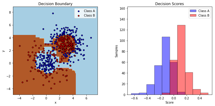
4.2 调用 Scikit Learn 的 AdaBoostClassifier 函数
例子来自 Two-class AdaBoost 。

print(__doc__)

# Author: Noel Dawe <noel.dawe@gmail.com>
#
# License: BSD 3 clause

import numpy as np
import matplotlib.pyplot as plt

from sklearn.ensemble import AdaBoostClassifier
from sklearn.tree import DecisionTreeClassifier
from sklearn.datasets import make_gaussian_quantiles


# Construct dataset
X1, y1 = make_gaussian_quantiles(cov=2.,
                                 n_samples=200, n_features=2,
                                 n_classes=2, random_state=1)
X2, y2 = make_gaussian_quantiles(mean=(3, 3), cov=1.5,
                                 n_samples=300, n_features=2,
                                 n_classes=2, random_state=1)
X = np.concatenate((X1, X2))
y = np.concatenate((y1, - y2 + 1))

# Create and fit an AdaBoosted decision tree
bdt = AdaBoostClassifier(DecisionTreeClassifier(max_depth=1),
                         algorithm="SAMME",
                         n_estimators=200)

bdt.fit(X, y)

plot_colors = "br"
plot_step = 0.02
class_names = "AB"

plt.figure(figsize=(10, 5))

# Plot the decision boundaries
plt.subplot(121)
x_min, x_max = X[:, 0].min() - 1, X[:, 0].max() + 1
y_min, y_max = X[:, 1].min() - 1, X[:, 1].max() + 1
xx, yy = np.meshgrid(np.arange(x_min, x_max, plot_step),
                     np.arange(y_min, y_max, plot_step))

Z = bdt.predict(np.c_[xx.ravel(), yy.ravel()])
Z = Z.reshape(xx.shape)
cs = plt.contourf(xx, yy, Z, cmap=plt.cm.Paired)
plt.axis("tight")

# Plot the training points
for i, n, c in zip(range(2), class_names, plot_colors):
    idx = np.where(y == i)
    plt.scatter(X[idx, 0], X[idx, 1],
                c=c, cmap=plt.cm.Paired,
                s=20, edgecolor='k',
                label="Class %s" % n)
plt.xlim(x_min, x_max)
plt.ylim(y_min, y_max)
plt.legend(loc='upper right')
plt.xlabel('x')
plt.ylabel('y')
plt.title('Decision Boundary')

# Plot the two-class decision scores
twoclass_output = bdt.decision_function(X)
plot_range = (twoclass_output.min(), twoclass_output.max())
plt.subplot(122)
for i, n, c in zip(range(2), class_names, plot_colors):
    plt.hist(twoclass_output[y == i],
             bins=10,
             range=plot_range,
             facecolor=c,
             label='Class %s' % n,
             alpha=.5,
             edgecolor='k')
x1, x2, y1, y2 = plt.axis()
plt.axis((x1, x2, y1, y2 * 1.2))
plt.legend(loc='upper right')
plt.ylabel('Samples')
plt.xlabel('Score')
plt.title('Decision Scores')

plt.tight_layout()
plt.subplots_adjust(wspace=0.35)
plt.show()

运行代码，获得的决策边界和得分情况如以下两幅图所示：

参考和拓展：
李航：《统计学习方法》；lihang_algorithms
Adaboost入门教程——最通俗易懂的原理介绍（图文实例） AdaboostExample
Machine-Learning-in-Action-Python3：《机器学习实战》python3 源码
adaboost：Simple Python Adaboost Implementation
adaboost-implementation：Implementation of AdaBoost algorithm in Python
AdaBoost：Small and easy C++ AdaBoost Implementation
FaceDetection：Human Face Detection based on AdaBoost
Naive_Bayes_Meet_Adaboost：Implement Naive Bayes and Adaboost from scratch and use them filter spam emails.

ViolinLeeChan

关注

0
点赞
踩
15

收藏

觉得还不错? 一键收藏
0
评论
AdaBoost 算法基础（二分类）

所属知识点：Machine Learning：Boosting 归纳和总结机器学习技术的库：ViolinLee/ML_notes。该库主要内容是我的机器学习笔记，同时挑选和收集各类与机器学习技术相关的高质量资源，欢迎大家关注和Star！会一直更新下去。微信公众号：“RoboticsCV”（微信号：ModernRobotics）。公众号专注机器人学，关注机器学习、计算机视觉等前沿技术在机器人领域中的...
复制链接

扫一扫

专栏目录