【深度学习从零开始】

动手学深度学习系列-自学笔记

1. 线性回归
   内容包括：数据流水线，模型，损失函数，小批量随机梯度下降优化器
2. 理论
   公式：y=wX+b 其中 w,b为参数 需要学习更新
   如何更新？
   计算梯度 g（求偏导）
   更新参数（w，b）（t+1）=(w,b)(t)-ug 这里的u为学习率，步长，步长不能太大，不能太小，太大容易错过最优值，太小收敛速度慢
3. 代码实现

#1.导入模块
%matplotlib inline
import random
import torch
from d2l import torch as d2l
#2.制作数据集
def synthetic_data(w,b,num_examples):
    X = torch.normal(0,1,(num_examples,len(w)))
   #normal函数是高斯概率密度函数，均值0，方差为1，size（样本个数，w一样的列）
    y = torch.matmul(X,w)+b #y=w*x+b
    y += torch.normal(0,0.01,y.shape)
    return X,y.reshape((-1,1))
true_w = torch.tensor([2,-3.4])
true_b = 4.2 

features,labels =synthetic_data(true_w,true_b,1000)#features是根据真实参数构造的X，lables是构造的y
print('features:',features[0],'\nlabel:',labels[0])
features:torch.tensor([-0.7677,1.8605])
label:torch.tensor([-3.6775])
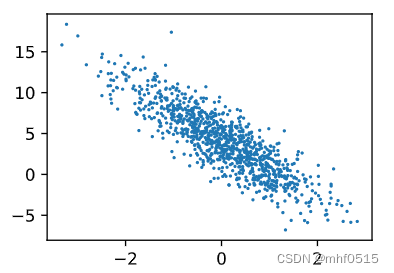
d2l.set_figsize()
d2l.plt.scatter(features[:,(1)].detach().numpy(),labels.detach().numpy(),1);

运行结果
features: tensor([ 0.1202, -0.9964])
label: tensor([7.8179])

补充：
Pyhton 中 shuffle()
Shuffle()方法将序列的所有元素随机排序
Shuffle（）是不能直接访问的，需要导入random()模块，然后通过random静态对象调用该方法，例如

import random
indices = list(range(10))
random.shuffle(indices)
indices

运行结果：[7, 0, 4, 9, 5, 6, 8, 2, 1, 3]

#3.批量处理数据
def data_iter(batch_size,features,labels):
    num_examples = len(features)
    indices = list(range(num_examples))
    random.shuffle(indices)
    for i in range(0,num_examples,batch_size):
        batch_indices = torch.tensor(indices[
            i:min(i+batch_size,num_examples)])
        yield features[batch_indices],labels[batch_indices]
        
batch_size=10
for X,y in data_iter(batch_size,features,labels):
    print(X,'\n',y)
    break

运行结果：
tensor([[ 0.5250, -0.2252],
[-1.1883, 0.1855],
[-0.2713, -0.1180],
[-0.0915, -0.9127],
[ 0.2781, -0.1090],
[-0.3397, 1.5661],
[-1.7854, 0.7900],
[-0.0486, 0.5448],
[-0.6125, 0.0115],
[ 0.5019, -1.1496]])
tensor([[ 6.0239],
[ 1.1922],
[ 4.0740],
[ 7.1077],
[ 5.1296],
[-1.8102],
[-2.0597],
[ 2.2431],
[ 2.9290],
[ 9.1216]])

#4.定义初始化，随机初始化参数w，b初始化为0
w = torch.normal(0,0.01,size=(2,1),requires_grad=True)
b = torch.zeros(1,requires_grad=True)
#5.定义损失函数
def linreg(X,w,b):
    return torch.matmul(X,w)+b     #y=w*x+b
def squrared_loss(y_hat,y):#将真实值y的形状转换为预测值y_hat的形状相同
    return (y_hat -y.reshape(y_hat.shape))**2/2   # MSE均方损失函数0.5*（y-y'）^2
    

#6.优化算法
def sgd(params,lr,batch_size):#随机梯度下降更新
    with torch.no_grad():#朝着减少损失的方向更新参数。
    # with torch.no_grad()  用于停止autograd模块的工作，
        for param in params:
            param -= lr*param.grad/batch_size #学习率lr ， batch_size 规范化步长
            #用param = param - lr * param.grad / batch_size
            #会导致导数丢失，下面的zero_()函数报错
            param.grad.zero_()

#7.训练
lr=0.03 #学习率
num_epochs=3 #迭代周期个数
net = linreg 
loss = squrared_loss

for epoch in range(num_epochs):
    for X,y in data_iter(batch_size,features,labels):# data_iter 遍历整个数据集
        l = loss(net(X,w,b),y)
        l.sum().backward()
        sgd([w,b],lr,batch_size)#使用参数的梯度更新参数
    with torch.no_grad():
        train_l = loss(net(features,w,b),labels)
        print(f'epoch {epoch+1},loss {float(train_l.mean()):f}')
#8.参看训练完的参数和真实参数的误差
print(f'w的估计误差：{true_w-w.reshape(true_w.shape)}')#真实的参数与训练学到的参数之间非常接近
print(f'b的估计误差:{true_b-b}')     

运行结果：
epoch 1,loss 0.000050
epoch 2,loss 0.000050
epoch 3,loss 0.000050
w的估计误差：tensor([-0.0004, -0.0006], grad_fn=)
b的估计误差:tensor([0.0001], grad_fn=)