


1.GRU
数据集(第一行是标题)(5639*9)
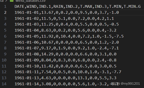
1.读取数据集
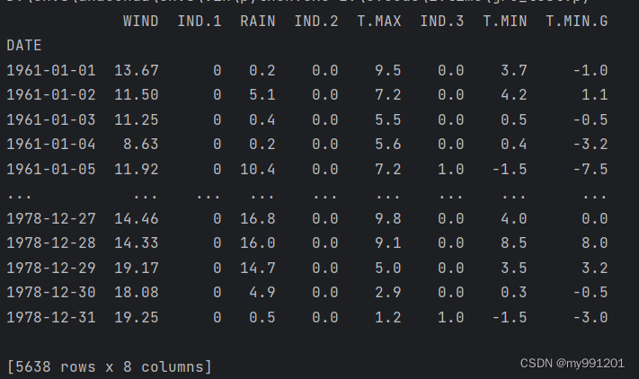
(5639*9)》(5638*8)第一行成了标题,第一列成了索引
df = pd.read_csv(config.data_path, index_col = 0)  # 用第一列做索引(5638*8)

print(df)![]()
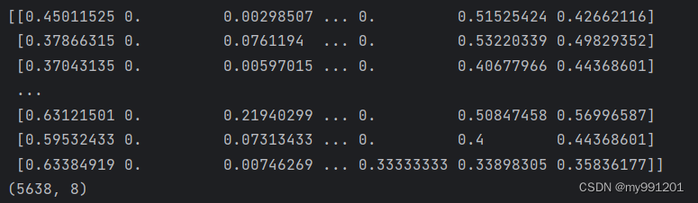
2.对数据标准化(划分到0-1之间)
scaler_model = MinMaxScaler()

data = scaler_model.fit_transform(np.array(df)) # 将 DataFrame df 中的所有数据进行标准化转换,并将结果保存到变量 data 中。

print(data)

print(data.shape) ![]()
3.获取训练数据 x_train: 170000,30,1 y_train:170000,7,1
# 形成训练数据,例如12345789 12-3456789
def split_data(data, timestep, feature_size):
dataX = [] # 保存X
dataY = [] # 保存Y
# 将整个窗口的数据保存到X中,将未来一天保存到Y中
for index in range(len(data) - timestep):
dataX.append(data[index: index + timestep][:, 0])
dataY.append(data[index + timestep][0])
dataX = np.array(dataX) # (5637,1)
dataY = np.array(dataY) # (5637,)
# 获取训练集大小
train_size = int(np.round(0.8 * dataX.shape[0])) # np.round:四舍五入,确保结果是整数。4510
# 划分训练集、测试集
x_train = dataX[: train_size, :].reshape(-1, timestep, feature_size) #(4510,1,1)
y_train = dataY[: train_size].reshape(-1, 1)# (4510,1)
x_test = dataX[train_size:, :].reshape(-1, timestep, feature_size) # (1127,1,1)
y_test = dataY[train_size:].reshape(-1, 1) # (1127,1)
return [x_train, y_train, x_test, y_test]
# 3.获取训练数据 x_train: 170000,30,1 y_train:170000,7,1
x_train, y_train, x_test, y_test = split_data(data, config.timestep, config.feature_size)
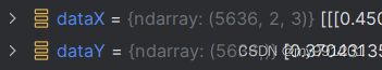
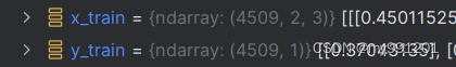
print(x_train)
print(y_train)若时间步是2,特征为3 (时间步是2,意思是前两天测下一天的)
数据里面一个特征和标签的样子:

这个是将数据集划分为特征和标签
划分训练和测试
一个时间步,一个特征的训练集,
 (3,1,1)
 (2,1)
(2,1)
两个时间步,一维特征。输入数据:(3,2,1)(样本数,时间步,每个时间步的特征数)
 输入数据:(3,2,1)
 标签(2,1)
4.将数据转为tensor
x_train_tensor = torch.from_numpy(x_train).to(torch.float32)
y_train_tensor = torch.from_numpy(y_train).to(torch.float32)
x_test_tensor = torch.from_numpy(x_test).to(torch.float32)
y_test_tensor = torch.from_numpy(y_test).to(torch.float32)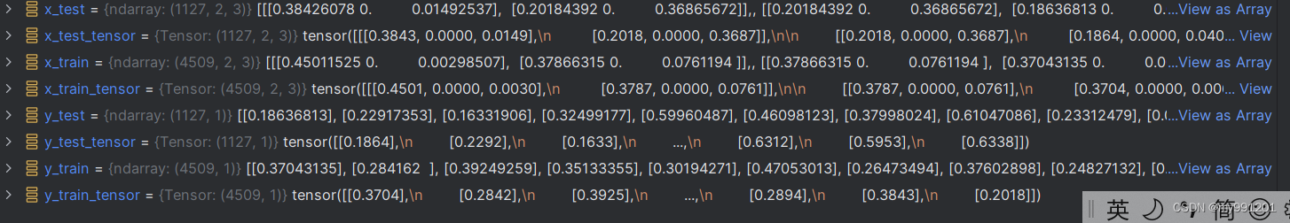
5.形成训练数据集
train_data = TensorDataset(x_train_tensor, y_train_tensor)
test_data = TensorDataset(x_test_tensor, y_test_tensor)
6.将数据加载成迭代器
train_loader = torch.utils.data.DataLoader(train_data,
                                           config.batch_size,
                                           False)

test_loader = torch.utils.data.DataLoader(test_data,
                                          config.batch_size,
                                          False)
7.定义模型
gru模型的参数:
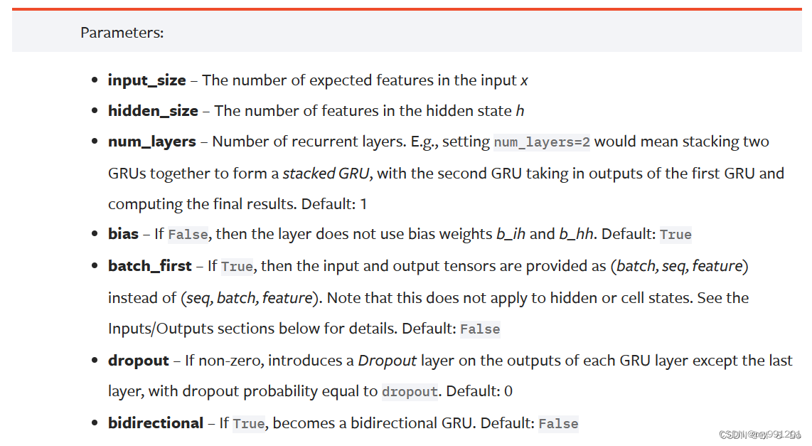
- input size: 每个时间点的特征维度,就是对应上面我们说的每天的特征维度是3还是1
- hidden size: GRU内部隐层的维度大小
- num layers: GRU的层数,默认为1
- bias: 是否在隐层中添加偏置bias,默认为True
- batch first: 如果设置为True, GRU的输入第一个维度为批次大小,也就是[batch size, seq len, feature size] ,如果为False,则模型的输入Tensor的维度为(seq len,batch size,feature size],默认为False
- dropout: 是否采用dropout
- bidirectional: 是否采用双向GRU模型,默认单向为False
模型输入:
 输入:(批次大小,时间步长度,特征数量)
GRU的模型输入Tensor的维度为 [batch size, seq len, feature size) ,其实也可以是 (seq len, batch size, feature size) ,但是我们常常将批次大小作为第一个维度传入,容易理解,本项目采用的输入维度为第一种方式,批次为先。
上处有小伙伴会存在一个问题,模型的输入还有一个 h 0作为输入,如果了解GRU原理的同学就可以知道这个输入变量是干嘛的,就是模型初始的隐层状态,对于这个变量可传可不传,如果不传则默认为0,有兴趣了解这个参数到底传入还是不传入可以参考这篇文章 对LSTM中每个batch都初始化隐含层的理解,本项目传入的隐层状态是传入的,但是传入的参数是以0进行填充,和默认不传入一致,只是为了让小伙伴了解这个参数是怎么传入的。
模型输出:()

输出:(批量大小,时间步,隐藏层节点数量*D)
GRU模型的输出有两个,一个输出的是模型的最终输出,也就是我们想要的输出,另外一个输出是模型的隐藏状态,对于本项目来说我们并不需要他。
对于这两个输出的维度一定要知道,首先是我们需要的输出 output ,该输出的维度为[batch size, seq len,D*hidden size],此处的D就是我们是否采用双向GRU,如果设置 bidirectional=True,则D=2,否则D=1,hidden size 就是GRU中间隐层的维度大小
对于 h n 的输出我们简答了解一下就好,因为我们不会对他进行处理为了能够理解GRU的输入和输出,举个例子说明:
import torch.nn as nn
import torch
model = nn.GRU(input_size=3, hidden_size=4, num_layers=2, batch_first=True)

# 我们定义了输入向量,该向量的维度为[4,5,3]
# ,分别代表[批次大小,时间片,特征大小]
# ,用语言叙述就是32个样本,然后用5
# 天的数据去未来1天的数据,每天的特征维度为3。
x = torch.randn(4, 5, 3)

print(x)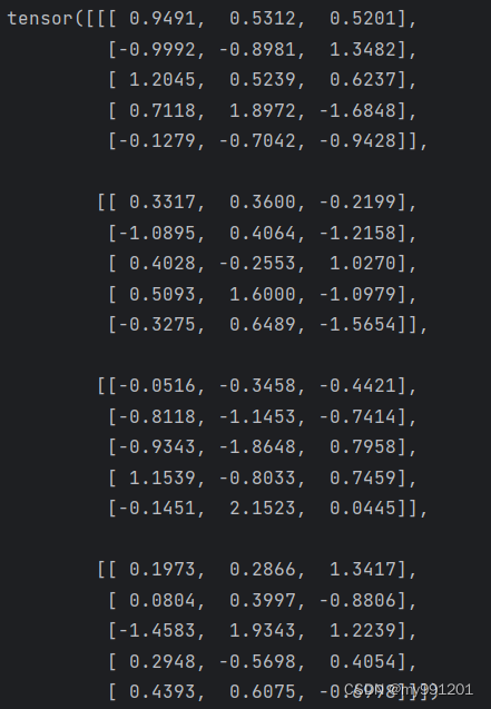
# 我们可以看到 output 的输出维度为[batch size, seq len, D* hidden size],由于我们的GRU是单向的,所以D=1。
output, h_0 = model(x)

print(output)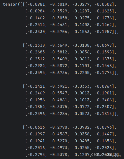

class GRU(nn.Module):
    def __init__(self, feature_size, hidden_size, num_layers, output_size):
        super(GRU, self).__init__()
        self.hidden_size = hidden_size  # 隐层大小
        self.num_layers = num_layers  # gru层数
        # feature_size为特征维度,就是每个时间点对应的特征数量,这里为1
        self.gru = nn.GRU(feature_size, hidden_size, num_layers, batch_first=True)
        # 当batch_first=True时,输入和输出张量的形状中批次大小(batch size)的维度将是第一个维度。例如,对于输入形状 (batch_size, sequence_length, input_size),如果batch_first=True,则意味着第一个维度是批次大小,即输入张量的形状是 (batch_size, sequence_length, input_size)。
        # 如果batch_first=False,那么默认情况下,输入张量的形状应该是 (sequence_length, batch_size, input_size),其中第一个维度是时间步,第二个维度是批次大小。
        self.fc = nn.Linear(hidden_size, output_size)

    def forward(self, x, hidden=None):
        batch_size = x.shape[0] # 获取批次大小

        # 初始化隐层状态
        if hidden is None:
            h_0 = x.data.new(self.num_layers, batch_size, self.hidden_size).fill_(0).float()
        else:
            h_0 = hidden

        # GRU运算
        output, h_0 = self.gru(x, h_0)

        # 获取GRU输出的维度信息(样本数,时间步,隐藏层大小)
        batch_size, timestep, hidden_size = output.shape

        # 将output变成 batch_size * timestep, hidden_dim
        output = output.reshape(-1, hidden_size) #这里就是把三维变成了二维,把第一维和第二维合并了

        # 全连接层
        output = self.fc(output)  # 输出形状为batch_size * timestep, 1

        # 转换维度,用于输出
        output = output.reshape(timestep, batch_size, -1)
        # 这样的话,是每块是一个时间步,我们只要最后一个时间步

        # 我们只需要返回最后一个时间片的数据即可
        return output[-1]
运行一个小批次的结果
 隐藏层状态:
1.h_0 = x.data.new(self.num_layers, batch_size, self.hidden_size).fill_(0).float()
在循环神经网络(RNN)和长短时记忆网络(LSTM)等循环层中,模型在处理时间序列数据时,每个时间步的隐层状态都是很重要的。h_0 是这个隐层状态的初始化值。
在前向传播的第一个时间步,通常将 h_0 设置为全零或者通过其他方式进行初始化。然后,在后续的时间步中,模型使用上一个时间步的隐层状态作为当前时间步的输入,这样模型可以捕捉到时间序列中的依赖关系。
在你提供的代码中,self.gru 是一个GRU层,它在每个时间步接收输入 x 和上一个时间步的隐层状态 h_0。这是因为 GRU(和其他循环层)是为了捕捉时间序列中的序列信息而设计的。
在第一个时间步,h_0 是一个初始化的隐层状态。在后续的时间步,h_0 就是前一个时间步的输出隐层状态,这样模型可以通过时间的推移学到序列中的模式和依赖关系。这也是循环神经网络的一个关键特性,使得它们能够有效处理时间序列数据。
2.模型的输入还有一个 h 0作为输入,如果了解GRU原理的同学就可以知道这个输入变量是干嘛的,就是模型初始的隐层状态,对于这个变量可传可不传,如果不传则默认为0,有兴趣了解这个参数到底传入还是不传入可以参考这篇文章 对LSTM中每个batch都初始化隐含层的理解,本项目传入的隐层状态是传入的,但是传入的参数是以0进行填充,和默认不传入一致,只是为了让小伙伴了解这个参数是怎么传入的。
model = GRU(config.feature_size, config.hidden_size, config.num_layers, config.output_size)  # 定义GRU网络
loss_function = nn.MSELoss()  # 定义损失函数
optimizer = torch.optim.AdamW(model.parameters(), lr=config.learning_rate)  # 定义优化器
8.模型训练
for epoch in range(config.epochs):
    model.train()
    running_loss = 0
    train_bar = tqdm(train_loader)  # 形成进度条
    for data in train_bar:
        x_train, y_train = data  # 解包迭代器中的X和Y
        optimizer.zero_grad() # 梯度清零
        y_train_pred = model(x_train) # 模型训练
        loss = loss_function(y_train_pred, y_train.reshape(-1, 1))
        loss.backward()
        optimizer.step()  # 梯度更新

        running_loss += loss.item()  # 将每一个小批次的损失相加
        train_bar.desc = "train epoch[{}/{}] loss:{:.3f}".format(epoch + 1,
                                                                 config.epochs,
                                                                 loss)

    # 模型验证  每一轮的时候又有验证
    model.eval()
    test_loss = 0
    with torch.no_grad():
        test_bar = tqdm(test_loader)
        for data in test_bar:
            x_test, y_test = data
            y_test_pred = model(x_test)
            test_loss = loss_function(y_test_pred, y_test.reshape(-1, 1))

    if test_loss < config.best_loss:
        config.best_loss = test_loss
        torch.save(model.state_dict(), config.save_path)

print('Finished Training')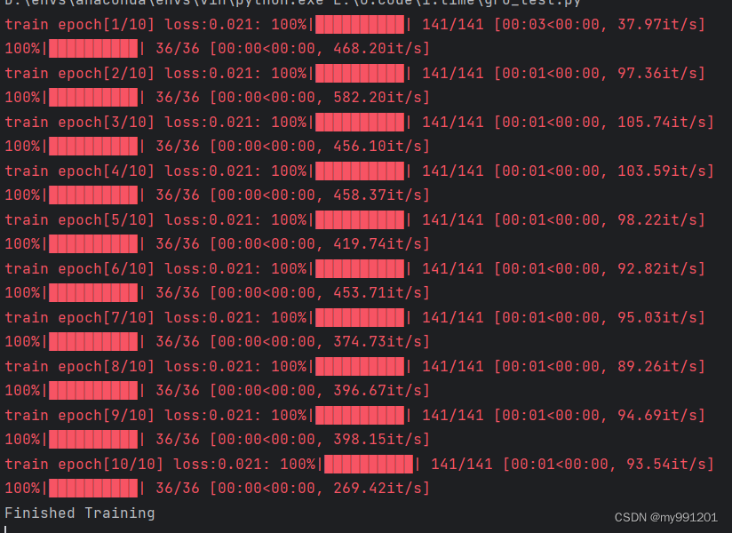
9.绘制结果
# 9.绘制结果
plot_size = 200
plt.figure(figsize=(12, 8))
plt.plot(scaler.inverse_transform((model(x_train_tensor).detach().numpy()[: plot_size]).reshape(-1, 1)), "b")
plt.plot(scaler.inverse_transform(y_train_tensor.detach().numpy().reshape(-1, 1)[: plot_size]), "r")
plt.legend()
plt.show()

y_test_pred = model(x_test_tensor)
plt.figure(figsize=(12, 8))
plt.plot(scaler.inverse_transform(y_test_pred.detach().numpy()[: plot_size]), "b")
plt.plot(scaler.inverse_transform(y_test_tensor.detach().numpy().reshape(-1, 1)[: plot_size]), "r")
plt.legend()
plt.show()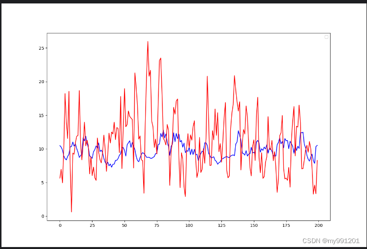
链接:
从这里学习,如有侵权立即删除。


 1330
1330


 被折叠的 条评论
为什么被折叠?
被折叠的 条评论
为什么被折叠?
 到【灌水乐园】发言


