


文章目录
Overview
- Dioptric cameras,通过透镜来实现,主要是折射
- Catadioptric cameras,使用一个标准相机加一个面镜(Shaped mirror)
- polydioptric camera,通过多个相机重叠视野
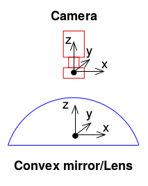
目前的视觉系统都是 central 的,入射光线会相交于同一点,点称为 single effective viewpoint。
全向相机 (omnidirectional camera )建模要考虑 mirror 反射或者鱼眼镜头折射。如下图所示。
Camera models
Pinhole
参数:
[
f
x
f
y
c
x
c
y
]
[f_x \ f_y \ c_x \ c_y]
[fx fy cx cy]
(1)
[
u
v
1
]
=
[
f
x
0
c
x
0
f
y
c
y
0
0
1
]
[
X
Z
Y
Z
1
]
\left[ \begin{array}{ccc} u \\ v \\ 1 \end{array} \right] =\begin{bmatrix} f_x & 0 & c_x \\ 0& f_y & c_y \\ 0&0&1 \end{bmatrix} \left[ \begin{array}{ccc} \frac{X}{Z} \\ \frac{Y}{Z} \\ 1 \end{array} \right] \tag{1}
⎣⎡uv1⎦⎤=⎣⎡fx000fy0cxcy1⎦⎤⎣⎡ZXZY1⎦⎤(1)
// cam2world
if(!distortion_)
  {
    xyz[0] = (u - cx_)/fx_;
    xyz[1] = (v - cy_)/fy_;
    xyz[2] = 1.0;
  }

// world2cam
  if(!distortion_)
  {
    px[0] = fx_*uv[0] + cx_;
    px[1] = fy_*uv[1] + cy_;
  }
omnidirectional
参数: [ ξ f x f y c x c y ] [ \xi \ \ f_x \ f_y \ c_x \ c_y] [ξ fx fy cx cy]
首先归一化
X
=
[
X
,
Y
,
Z
]
{\mathcal X} =[X, Y,Z]
X=[X,Y,Z]到球面上
(2)
[
X
s
Y
s
Z
s
]
=
X
∣
∣
X
∣
∣
\left[ \begin{array}{c} X_s \\ Y_s \\ Z_s \end{array} \right] =\frac{\mathcal X}{|| \mathcal X||} \tag{2}
⎣⎡XsYsZs⎦⎤=∣∣X∣∣X(2)
变换坐标系,并变换到归一化平面
(3)
m
u
=
(
X
s
Z
s
+
ξ
,
Y
s
Z
s
+
ξ
,
1
)
=
ℏ
(
X
s
)
\mathbf{m}_{u}=\left(\frac{X_{s}}{Z_{s}+\xi}, \frac{Y_{s}}{Z_{s}+\xi}, 1\right)=\hbar\left(\mathcal{X}_{s}\right) \tag{3}
mu=(Zs+ξXs,Zs+ξYs,1)=ℏ(Xs)(3)
然后可以加入畸变,这里先不考虑。
然后使用相机内参,和公式(1)一样:
(4)
[
u
v
1
]
=
[
f
x
0
c
x
0
f
y
c
y
0
0
1
]
m
u
\left[ \begin{array}{ccc} u \\ v \\ 1 \end{array} \right] =\begin{bmatrix} f_x & 0 & c_x \\ 0& f_y & c_y \\ 0&0&1 \end{bmatrix} \mathbf{m}_{u} \tag{4}
⎣⎡uv1⎦⎤=⎣⎡fx000fy0cxcy1⎦⎤mu(4)
其中公式(3)中的逆变换,即从图像系得到球面公式(2)公式为
(5)
ℏ
−
1
(
m
u
)
=
[
X
s
Y
s
Z
s
]
=
[
ξ
+
1
+
(
1
−
ξ
2
)
(
x
2
+
y
2
)
x
2
+
y
2
+
1
x
ξ
+
1
+
(
1
−
ξ
2
)
(
x
2
+
y
2
)
x
2
+
y
2
+
1
y
ξ
+
1
+
(
1
−
ξ
2
)
(
x
2
+
y
2
)
x
2
+
y
2
+
1
−
ξ
]
\hbar^{-1}\left(\mathbf{m}_{u}\right)=\left[ \begin{array}{c} X_s \\ Y_s \\ Z_s \end{array} \right] = \left[ \begin{array}{c}{\frac{\xi+\sqrt{1+\left(1-\xi^{2}\right)\left(x^{2}+y^{2}\right)}}{x^{2}+y^{2}+1} x} \\ {\frac{\xi+\sqrt{1+\left(1-\xi^{2}\right)\left(x^{2}+y^{2}\right)}}{x^{2}+y^{2}+1} y} \\ {\frac{\xi+\sqrt{1+\left(1-\xi^{2}\right)\left(x^{2}+y^{2}\right)}}{x^{2}+y^{2}+1}-\xi}\end{array}\right] \tag{5}
ℏ−1(mu)=⎣⎡XsYsZs⎦⎤=⎣⎢⎢⎢⎡x2+y2+1ξ+1+(1−ξ2)(x2+y2)xx2+y2+1ξ+1+(1−ξ2)(x2+y2)yx2+y2+1ξ+1+(1−ξ2)(x2+y2)−ξ⎦⎥⎥⎥⎤(5)
相应的得到归一化平面坐标为(比较奇怪的一个坐标):
(6)
[
X
s
Z
s
+
ξ
Y
s
Z
s
+
ξ
Z
s
Z
s
+
ξ
]
=
[
x
y
1
−
ξ
x
2
+
y
2
+
1
ξ
+
1
+
(
1
−
ξ
2
)
(
x
2
+
y
2
)
]
\left[ \begin{array}{c} \frac {X_s}{Z_s +\xi} \\ \frac {Y_s}{Z_s +\xi} \\ \frac {Z_s}{Z_s +\xi} \end{array} \right] =\left[ \begin{array}{c}{x} \\ {y} \\ {1-\xi \frac{x^{2}+y^{2}+1}{\xi+\sqrt{1+\left(1-\xi^{2}\right)\left(x^{2}+y^{2}\right)}}}\end{array}\right] \tag{6}
⎣⎢⎡Zs+ξXsZs+ξYsZs+ξZs⎦⎥⎤=⎣⎢⎡xy1−ξξ+1+(1−ξ2)(x2+y2)x2+y2+1⎦⎥⎤(6)
// cam2world
// 像素坐标变换到球面
mx_u = m_inv_K11 * p(0) + m_inv_K13;
my_u = m_inv_K22 * p(1) + m_inv_K23;

double xi = mParameters.xi();
if (xi == 1.0)
{
    lambda = 2.0 / (mx_u * mx_u + my_u * my_u + 1.0);
    P << lambda * mx_u, lambda * my_u, lambda - 1.0;
}
else
{
    lambda = (xi + sqrt(1.0 + (1.0 - xi * xi) * (mx_u * mx_u + my_u * my_u))) / (1.0 + mx_u * mx_u + my_u * my_u);
    P << lambda * mx_u, lambda * my_u, lambda - xi;
}


// 或者变换到归一化平面
if (xi == 1.0)
{
    P << mx_u, my_u, (1.0 - mx_u * mx_u - my_u * my_u) / 2.0;
}
else
{
    // Reuse variable
    rho2_d = mx_u * mx_u + my_u * my_u;
    P << mx_u, my_u, 1.0 - xi * (rho2_d + 1.0) / (xi + sqrt(1.0 + (1.0 - xi * xi) * rho2_d));
}

// 正向比较简单,按照公式来就行了,代码忽略

Distortion models
Equidistant (EQUI)
参数:
[
k
1
,
k
2
,
k
3
,
k
4
]
[k_1, \ k_2, \ k_3, \ k_4 ]
[k1, k2, k3, k4]
(7)
{
r
=
x
c
2
+
y
c
2
θ
=
atan
2
(
r
,
∣
z
c
∣
)
=
atan
2
(
r
,
1
)
=
atan
(
r
)
\left\{\begin{array}{l}{r=\sqrt{x_{c}^{2}+y_{c}^{2}}} \\ {\theta=\operatorname{atan} 2\left(r,\left|z_{c}\right|\right)=\operatorname{atan} 2(r, 1)=\operatorname{atan}(r)}\end{array}\right. \tag{7}
{r=xc2+yc2θ=atan2(r,∣zc∣)=atan2(r,1)=atan(r)(7)
另外:
f
=
r
′
⋅
tan
(
θ
)
f=r^{\prime} \cdot \tan (\theta) \quad
f=r′⋅tan(θ) where
r
′
=
u
2
+
v
2
\quad r^{\prime}=\sqrt{u^{2}+v^{2}}
r′=u2+v2
(8)
θ
d
=
θ
(
1
+
k
1
⋅
θ
2
+
k
2
⋅
θ
4
+
k
3
⋅
θ
6
+
k
4
⋅
θ
8
)
\theta_{d}=\theta\left(1+k_1 \cdot \theta^{2}+k_2 \cdot \theta^{4}+k_3 \cdot \theta^{6}+k_4 \cdot \theta^{8}\right) \tag{8}
θd=θ(1+k1⋅θ2+k2⋅θ4+k3⋅θ6+k4⋅θ8)(8)
(9) { x d = θ d ⋅ x c r y d = θ d ⋅ y c r \left\{\begin{array}{l}{x_{d}=\frac{\theta_{d} \cdot x_{c}}{r}} \\ {y_{d}=\frac{\theta_{d} \cdot y_{c}}{r}}\end{array}\right. \tag{9} {xd=rθd⋅xcyd=rθd⋅yc(9)
float ix = (x - ocx) / ofx;
float iy = (y - ocy) / ofy;
float r = sqrt(ix * ix + iy * iy);
float theta = atan(r);
float theta2 = theta * theta;
float theta4 = theta2 * theta2;
float theta6 = theta4 * theta2;
float theta8 = theta4 * theta4;
float thetad = theta * (1 + k1 * theta2 + k2 * theta4 + k3 * theta6 + k4 * theta8);
float scaling = (r > 1e-8) ? thetad / r : 1.0;
float ox = fx*ix*scaling + cx;
float oy = fy*iy*scaling + cy;
Radtan
参数:
[
k
1
,
k
2
,
p
1
,
p
2
]
[k_1, \ k_2, \ p_1, \ p_2 ]
[k1, k2, p1, p2]
(10)
{
x
distorted
=
x
(
1
+
k
1
r
2
+
k
2
r
4
)
+
2
p
1
x
y
+
p
2
(
r
2
+
2
x
2
)
y
distorted
=
y
(
1
+
k
1
r
2
+
k
2
r
4
)
+
p
1
(
r
2
+
2
y
2
)
+
2
p
2
x
y
\left\{\begin{array}{l}{x_{\text { distorted }}=x\left(1+k_{1} r^{2}+k_{2} r^{4}\right)+2 p_{1} x y+p_{2}\left(r^{2}+2 x^{2}\right)} \\ {y_{\text { distorted }}=y\left(1+k_{1} r^{2}+k_{2} r^{4}\right)+p_{1}\left(r^{2}+2 y^{2}\right)+2 p_{2} x y}\end{array}\right. \tag{10}
{x distorted =x(1+k1r2+k2r4)+2p1xy+p2(r2+2x2)y distorted =y(1+k1r2+k2r4)+p1(r2+2y2)+2p2xy(10)
其中
x
,
y
x,y
x,y是不带畸变的坐标,
x
d
i
s
t
o
r
t
e
d
,
y
d
i
s
t
o
r
t
e
d
x_{distorted}, y_{distorted}
xdistorted,ydistorted是有畸变图像的坐标。
// cam2world(distorted2undistorted)
// 先经过内参变换,再进行畸变矫正
{
  cv::Point2f uv(u,v), px;
  const cv::Mat src_pt(1, 1, CV_32FC2, &uv.x);
  cv::Mat dst_pt(1, 1, CV_32FC2, &px.x);
  cv::undistortPoints(src_pt, dst_pt, cvK_, cvD_);
  xyz[0] = px.x;
  xyz[1] = px.y;
  xyz[2] = 1.0;
}
// 先经过镜头发生畸变,再成像过程,乘以内参
// world2cam(undistorted2distorted)
{
  double x, y, r2, r4, r6, a1, a2, a3, cdist, xd, yd;
  x = uv[0];
  y = uv[1];
  r2 = x*x + y*y;
  r4 = r2*r2;
  r6 = r4*r2;
  a1 = 2*x*y;
  a2 = r2 + 2*x*x;
  a3 = r2 + 2*y*y;
  cdist = 1 + d_[0]*r2 + d_[1]*r4 + d_[4]*r6;
  xd = x*cdist + d_[2]*a1 + d_[3]*a2;
  yd = y*cdist + d_[2]*a3 + d_[3]*a1;
  px[0] = xd*fx_ + cx_;
  px[1] = yd*fy_ + cy_;
}
FOV
参数:
[
ω
]
[\omega]
[ω]
(11)
{
x
d
i
s
t
o
r
t
e
d
=
r
d
r
⋅
x
y
d
i
s
t
o
r
t
e
d
=
r
d
r
⋅
y
\left\{\begin{array}{l} {x_{distorted}=\frac{r_{d}}{r} \cdot x } \\ {y_{distorted}=\frac{r_{d}}{r} \cdot y } \end{array} \right. \tag{11}
{xdistorted=rrd⋅xydistorted=rrd⋅y(11)
其中
(12)
r
d
=
1
ω
arctan
(
2
⋅
r
⋅
tan
(
ω
2
)
)
r
=
(
X
Z
)
2
+
(
Y
Z
)
2
=
x
2
+
y
2
r_{d}=\frac{1}{\omega} \arctan \left(2 \cdot r \cdot \tan \left(\frac{\omega}{2}\right)\right) \\ r=\sqrt{{\left(\frac{X}{Z}\right)}^{2}+{\left(\frac{Y}{Z}\right)}^{2}}=\sqrt{x^2+y^2} \tag{12}
rd=ω1arctan(2⋅r⋅tan(2ω))r=(ZX)2+(ZY)2=x2+y2(12)
// cam2world(distorted2undistorted)
Vector2d dist_cam( (x - cx_) * fx_inv_, (y - cy_) * fy_inv_ );
double dist_r = dist_cam.norm();
double r = invrtrans(dist_r);
double d_factor;
if(dist_r > 0.01)
  d_factor =  r / dist_r;
else
  d_factor = 1.0;
return unproject2d(d_factor * dist_cam).normalized();


// world2cam(undistorted2distorted)
double r = uv.norm();
double factor = rtrans_factor(r);
Vector2d dist_cam = factor * uv;
return Vector2d(cx_ + fx_ * dist_cam[0],
                  cy_ + fy_ * dist_cam[1]);

// 函数
//! Radial distortion transformation factor: returns ration of distorted / undistorted radius.
inline double rtrans_factor(double r) const
{
  if(r < 0.001 || s_ == 0.0)
    return 1.0;
  else
    return (s_inv_* atan(r * tans_) / r);
};

//! Inverse radial distortion: returns un-distorted radius from distorted.
inline double invrtrans(double r) const
{
  if(s_ == 0.0)
    return r;
  return (tan(r * s_) * tans_inv_);
};
Projection model
Full projection model
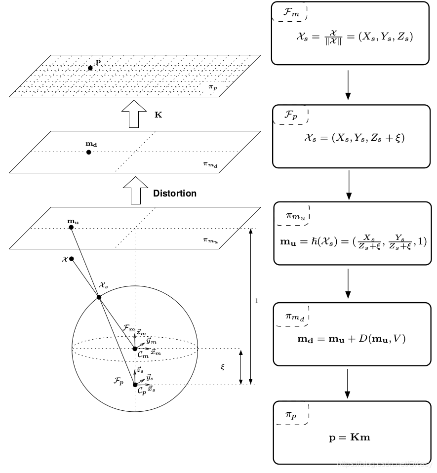
- 第一步是将mirror系下的世界坐标点投影到归一化球面(unit sphere)
(13) ( X ) F m → ( X s ) F m = X ∥ X ∥ = ( X s , Y s , Z s ) (\mathcal{X})_{\mathcal{F}_{m}} \rightarrow\left(\mathcal{X}_{s}\right)_{\mathcal{F}_{m}}=\frac{\mathcal{X}}{\|\mathcal{X}\|}=\left(X_{s}, Y_{s}, Z_{s}\right) \tag{13} (X)Fm→(Xs)Fm=∥X∥X=(Xs,Ys,Zs)(13)
- 将投影点的坐标变换到一个新坐标系下表示,新坐标系的原点位于 C p = ( 0 , 0 , ξ ) \mathcal{C}_{p}=(0,0, \xi) Cp=(0,0,ξ)
(14) ( X s ) F m → ( X s ) F p = ( X s , Y s , Z s + ξ ) \left(\mathcal{X}_{s}\right)_{\mathcal{F}_{m}} \rightarrow\left(\mathcal{X}_{s}\right)_{\mathcal{F}_{p}}=\left(X_{s}, Y_{s}, Z_{s}+\xi\right)\tag{14} (Xs)Fm→(Xs)Fp=(Xs,Ys,Zs+ξ)(14)
- 将其投影到归一化平面
(15) m u = ( X s Z s + ξ , Y s Z s + ξ , 1 ) = ℏ ( X s ) \mathbf{m}_{u}=\left(\frac{X_{s}}{Z_{s}+\xi}, \frac{Y_{s}}{Z_{s}+\xi}, 1\right)=\hbar\left(\mathcal{X}_{s}\right)\tag{15} mu=(Zs+ξXs,Zs+ξYs,1)=ℏ(Xs)(15)
- 增加畸变影响
(16) m d = m u + D ( m u , V ) \mathbf{m}_{d}=\mathbf{m}_{u}+D\left(\mathbf{m}_{u}, V\right)\tag{16} md=mu+D(mu,V)(16)
- 乘上相机模型内参矩阵 K \bf K K,其中 γ \gamma γ表示焦距, ( u 0 , v 0 ) (u_0,v_0) (u0,v0)表示光心, s s s表示坐标系倾斜系数, r r r表示纵横比
(17) p = K m = [ γ γ s u 0 0 γ r v 0 0 0 1 ] m = k ( m ) \mathbf{p}=\mathbf{K} \mathbf{m}=\left[ \begin{array}{ccc}{\gamma} & {\gamma s} & {u_{0}} \\ {0} & {\gamma r} & {v_{0}} \\ {0} & {0} & {1}\end{array}\right] \mathbf{m}=k(\mathbf{m})\tag{17} p=Km=⎣⎡γ00γsγr0u0v01⎦⎤m=k(m)(17)
下图是相机焦距与面镜类型的参数对比。

MEI Camera
Omni + Radtan6
Pinhole Camera
Pinhole + Radtan
atan Camera
Pinhole + FOV
Davide Scaramuzza Camera
参数: [ P o l y [ N ] , C , D , E , x c , y c ] [Poly[N], \ C, \ D, \ E, \ x_c, \ y_c] [Poly[N], C, D, E, xc, yc]
这个是ETHZ的工作7,畸变和相机内参放在一起了,为了克服针对鱼眼相机参数模型的知识缺乏,使用一个多项式来代替。
直接上代码吧:
// ************************** world2cam **************************
Vector2d uv;

// transform world-coordinates to Davide's camera frame
Vector3d worldCoordinates_bis;
worldCoordinates_bis[0] = xyz_c[1];
worldCoordinates_bis[1] = xyz_c[0];
worldCoordinates_bis[2] = -xyz_c[2];

double norm = sqrt( pow( worldCoordinates_bis[0], 2 ) + pow( worldCoordinates_bis[1], 2 ) );
double theta = atan( worldCoordinates_bis[2]/norm );

// Important: we exchange x and y since Pirmin's stuff is working with x along the columns and y along the rows,
// Davide's framework is doing exactly the opposite
double rho;
double t_i;
double x;
double y;

if(norm != 0)
{
  rho = ocamModel.invpol[0];

  t_i = 1;
  // 多项式畸变
  for( int i = 1; i < ocamModel.length_invpol; i++ )
  {
    t_i *= theta;
    rho += t_i * ocamModel.invpol[i];
  }

  x = worldCoordinates_bis[0] * rho/norm;
  y = worldCoordinates_bis[1] * rho/norm;

  //? we exchange 0 and 1 in order to have pinhole model again
  uv[1] = x * ocamModel.c + y * ocamModel.d + ocamModel.xc;
  uv[0] = x * ocamModel.e + y + ocamModel.yc;
}
else
{
  // we exchange 0 and 1 in order to have pinhole model again
  uv[1] = ocamModel.xc;
  uv[0] = ocamModel.yc;
}


//******************** cam2world ******************
double invdet  = 1 / ( ocamModel.c - ocamModel.d * ocamModel.e );

xyz[0] = invdet * ( ( v - ocamModel.xc ) - ocamModel.d * ( u - ocamModel.yc ) );
xyz[1] = invdet * ( -ocamModel.e * ( v - ocamModel.xc ) + ocamModel.c * ( u - ocamModel.yc ) );

double r = sqrt(  pow( xyz[0], 2 ) + pow( xyz[1], 2 ) ); //distance [pixels] of  the point from the image center
xyz[2] = ocamModel.pol[0];
double r_i = 1;

for( int i = 1; i < ocamModel.length_pol; i++ )
{
  r_i *= r;
  xyz[2] += r_i * ocamModel.pol[i];
}

xyz.normalize();

// change back to pinhole model:
double temp = xyz[0];
xyz[0] = xyz[1];
xyz[1] = temp;
xyz[2] = -xyz[2];
Examples
据大佬说,根据经验,小于90度使用Pinhole,大于90度使用MEI模型。
要注意畸变矫正之后的相机内参会变化。
DSO:Pinhole + Equi / Radtan / FOV
VINS:Pinhole / Omni + Radtan
SVO:Pinhole / atan / Scaramuzza
OpenCV:cv: pinhole + Radtan , cv::fisheye: pinhole + Equi , cv::omnidir: Omni + Radtan
C++ Code
Reference
https://blog.csdn.net/zhangjunhit/article/details/89137958 ↩︎
https://blog.csdn.net/u011178262/article/details/86656153#OpenCV_fisheye_camera_model_61 ↩︎
Mei C, Rives P. Single view point omnidirectional camera calibration from planar grids[C]//Proceedings 2007 IEEE International Conference on Robotics and Automation. IEEE, 2007: 3945-3950. ↩︎
Kneip L, Scaramuzza D, Siegwart R. A novel parametrization of the perspective-three-point problem for a direct computation of absolute camera position and orientation[C]//CVPR 2011. IEEE, 2011: 2969-2976. ↩︎


 1404
1404

 被折叠的 条评论
为什么被折叠?
被折叠的 条评论
为什么被折叠?
 到【灌水乐园】发言


