


文章目录
简介
Martin Arjovsky, Soumith Chintala, Leon Bottou, Wasserstein GAN, arXiv prepring, 2017
Ishaan Gulrajani, Faruk Ahmed,Martin Arjovsky, Vincent Dumoulin, Aaron Courville, “Improved Training of Wasserstein GANs”,arXiv prepring,2017
这节讲GAN的优化。
公式输入请参考:在线Latex公式
JS divergence来衡量分布的问题
JS divergence is not suitable. 原因在于:
In most cases,
P
G
P_G
PG and
P
d
a
t
a
P_{data}
Pdata are not overlapped.
就是生成的数据和真实数据是不重叠的。不重叠有两方面的原因:
1、数据本身的问题The nature of data
Both
P
d
a
t
a
P_{data}
Pdata and
P
G
P_G
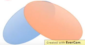
PG are low-dim manifold in high-dim space.The overlap can be ignored.
例如:图片是高(三)维空间中的低(二)维空间的manifold。
如下图所示,可以看到两个曲线overlap的部分是很小的。

2、采样Sampling的原因
尽管数据本来是有overlap,但是我们不是取所有的数据:
Even though
P
d
a
t
a
P_{data}
Pdata and
P
G
P_G
PG have overlap.
我们是对这两堆分布进行采样,我们不会采样全部,而是部分:
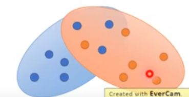
以上两个分布采样的结果是不会有overlap的,除非你采样超多点,因此这两个采样结果可以看做是两个不同的分布:

也就是说If you do not have enough sampling ……结果就是没有重合。
没有重合的时候,用JS divergence来衡量分布,会发生什么?
What is the problem of JS divergence?
只要两个分布不重合,那么算出来的结果都一样:
l
o
g
2
log2
log2
JS divergence is
l
o
g
2
log2
log2 if two distributions do not overlap

按理说
P
G
1
P_{G_1}
PG1要比
P
G
0
P_{G_0}
PG0好,因为它比
P
G
0
P_{G_0}
PG0要更加接近
P
d
a
t
a
P_{data}
Pdata,JS divergence都一样,除非二者重合,两个才会有JS divergence=0。这样在不重合的状态下是没有办法做优化(train)的。
结果为什么会是:
l
o
g
2
log2
log2?
Intuition: If two distributions do not overlap, binary classifier achieves 100% accuracy.
用一个二分类的分类器对不重叠的两个分布做分类,总是可以得到100%的准确率,因此其cost都是一样的。
Same objective value is obtained. →Same divergence.
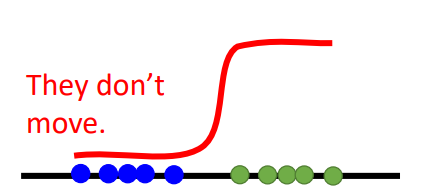
因此在GAN中用二分类来训练是很难收敛的。例如:
用绿色点代表真实数据
蓝色点代表生成数据
如果是一个sigmoid函数的话,可以看到蓝色点这块的梯度都是0,所以在GD的时候是不会更新(动)的。所以有人提出说,不要把这个分类函数训练得太好,使得整个分类函数在蓝色点部分有梯度,这样才可以进行梯度更新,但是这个训练得好不好(太用力,没梯度,不够用力,discriminator无法工作),很难把握。
因此为了做GAN的优化,出现了LSGAN
Least Square GAN (LSGAN)
算法思想就是用线性分类器替换sigmoid分类器。也就是把分类问题换成了回归问题。
Replace sigmoid with linear (replace classification with regression)

train的目标是使得真实数据越接近1越好,生成数据越接近0越好。
Wasserstein GAN (WGAN): Earth Mover’s Distance
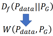
Wasserstein中a发[æ]的音,思想就是不用JS divergence来衡量两个分布的差别,而是用另外一个方法:Earth Mover’s Distance。这个玩意的概念很土。。。
把P和Q看作是两堆土,而你是蓝翔毕业的挖掘机(Earth Mover)司机,要把P这堆土(原文是挖到Q那里,但是应该不是这个意思)挖成Q的形状,而Earth Mover’s Distance就是挖掘机来回移动的平均距离。
• Considering one distribution P as a pile of earth, and another distribution Q as the target
• The average distance the earth mover has to move the earth.

上面的分布是简化了的,土堆应该是这样:

要把P变成Q,可以有很多种挖法:

上图中的左边是是把邻近的土进行移动,右边是比较远的土进行移动。我们一般用左边的那种。
There many possible “moving plans”.
Using the “moving plan” with the smallest average distance to define the earth mover’s distance.
Best “moving plans” of this example

正式的定义:
A “moving plan” is a matrix. The value of the element is the amount of earth from one position to another.
Average distance of a plan
γ
\gamma
γ:
B
(
γ
)
=
∑
x
p
,
x
q
γ
(
x
p
,
x
q
)
∣
∣
x
p
−
x
q
∣
∣
B(\gamma)=\sum_{x_p,x_q}\gamma(x_p,x_q)||x_p-x_q||
B(γ)=xp,xq∑γ(xp,xq)∣∣xp−xq∣∣
Earth Mover’s Distance:
W
(
P
,
Q
)
=
m
i
n
γ
∈
∏
B
(
γ
)
W(P,Q)=\underset{\gamma\in\prod}{min}B(\gamma)
W(P,Q)=γ∈∏minB(γ)
这个矩阵中某个点(x,y)代表从行x移动多少土到列y,这个点的颜色越亮,那么代表移动的土越多。
行x所有点加起来,对应P中对应第x堆土;
列y所有点加起来,对应Q中对应第y堆土。
给定矩阵(确定移动方案后)
γ
\gamma
γ,计算移动距离
B
(
γ
)
B(\gamma)
B(γ),如上面公式所示,然后穷举所有移动方案,找到最小那个。

也就是说这个方法要接一个优化方案后才能得到解。
Why Earth Mover’s Distance?
用Earth Mover’s Distance来替换JS divergence
那么也就改善了之前两个分布不重叠无法更新梯度的缺点:

可以看到d50比d0是有进步的,所以梯度才能不断更新迭代,最后到达两个分布距离为0的目标。
WGAN
如何用wasserstein distance来衡量两个分布,这个过程的证明比较复杂,直接给结论:
Evaluate wasserstein distance between
P
d
a
t
a
P_{data}
Pdata and
P
G
P_G
PG
V
(
G
,
D
)
=
m
a
x
D
∈
1
−
L
i
p
s
c
h
i
t
z
{
E
x
∼
P
d
a
t
a
[
D
(
x
)
]
−
E
x
∼
P
G
[
D
(
x
)
]
}
V(G,D)=\underset{D\in 1-Lipschitz}{max}\{E_{x\sim P_{data}}[D(x)]-E_{x\sim P_{G}}[D(x)]\}
V(G,D)=D∈1−Lipschitzmax{Ex∼Pdata[D(x)]−Ex∼PG[D(x)]}
公式的意思是:如果x是从
P
d
a
t
a
P_{data}
Pdata 采样出来的,希望他的Discriminator值越大越好,如果是从
P
G
P_G
PG采样出来的,希望他的Discriminator值越小越好,另外还有一个约束就是D要是一个
1
−
L
i
p
s
c
h
i
t
z
1-Lipschitz
1−Lipschitz的函数(啥意思后面讲,就是要D越平滑越好)
为什么要平滑呢,如果没有平滑的这个限制:

D就会在生成数据
P
d
a
t
a
P_{data}
Pdata的地方趋向于负无穷大,在真实数据
P
G
P_G
PG的地方趋向于正无穷大。两个分布就会差很多。加入平滑限制,会使得D不会无限的上升和下降,会停在某个地方。
L
i
p
s
c
h
i
t
z
F
u
n
c
t
i
o
n
Lipschitz\space Function
Lipschitz Function
∣
∣
f
(
x
1
)
−
f
(
x
2
)
∣
∣
≤
K
∣
∣
x
1
−
x
2
∣
∣
||f(x_1)-f(x_2)||\leq K||x_1-x_2||
∣∣f(x1)−f(x2)∣∣≤K∣∣x1−x2∣∣
可以看到公式左边是输出的变化,右边是输入的变化,也就是说输出的变化要小于K倍的输入的变化。
当K=1,我们就把这个满足这个不等式的函数称为
1
−
L
i
p
s
c
h
i
t
z
1-Lipschitz
1−Lipschitz
也就是
∣
∣
f
(
x
1
)
−
f
(
x
2
)
∣
∣
≤
∣
∣
x
1
−
x
2
∣
∣
||f(x_1)-f(x_2)||\leq ||x_1-x_2||
∣∣f(x1)−f(x2)∣∣≤∣∣x1−x2∣∣
也就是不会变化很快。例如下面的绿色函数比较像
1
−
L
i
p
s
c
h
i
t
z
F
u
n
c
t
i
o
n
1-Lipschitz\space Function
1−Lipschitz Function,蓝色函数就肯定不是
1
−
L
i
p
s
c
h
i
t
z
F
u
n
c
t
i
o
n
1-Lipschitz\space Function
1−Lipschitz Function

如何满足
1
−
L
i
p
s
c
h
i
t
z
F
u
n
c
t
i
o
n
1-Lipschitz\space Function
1−Lipschitz Function约束条件呢?原论文使用的方法是:Weight Clipping
Force the parameters
w
w
w between
c
c
c and
−
c
-c
−c. After parameter update,
if w > c, w = c;
if w < -c, w = -c
这个方法很简单,其实用这个方法弄出来的函数并不满足
1
−
L
i
p
s
c
h
i
t
z
F
u
n
c
t
i
o
n
1-Lipschitz\space Function
1−Lipschitz Function约束条件,但是基本能work,能达到使得D平滑的目的。也是没有办法的办法,因为
1
−
L
i
p
s
c
h
i
t
z
F
u
n
c
t
i
o
n
1-Lipschitz\space Function
1−Lipschitz Function不好优化。
Improved WGAN (WGAN-GP)
对Weight Clipping进行改进,函数还是一样:
V
(
G
,
D
)
=
m
a
x
D
∈
1
−
L
i
p
s
c
h
i
t
z
{
E
x
∼
P
d
a
t
a
[
D
(
x
)
]
−
E
x
∼
P
G
[
D
(
x
)
]
}
V(G,D)=\underset{D\in 1-Lipschitz}{max}\{E_{x\sim P_{data}}[D(x)]-E_{x\sim P_{G}}[D(x)]\}
V(G,D)=D∈1−Lipschitzmax{Ex∼Pdata[D(x)]−Ex∼PG[D(x)]}
但是Improved WGAN对于约束换了一个角度,就是梯度的norm要小于等于1。
A differentiable function is 1-Lipschitz if and only if it has gradients with norm less than or equal to 1 everywhere.
这个转换和之前的约束是一样的。

关于norm的计算是有一个近似计算的方法的:
V
(
G
,
D
)
≈
m
a
x
D
{
E
x
∼
P
d
a
t
a
[
D
(
x
)
]
−
E
x
∼
P
G
[
D
(
x
)
]
−
λ
∫
x
m
a
x
(
0
,
∣
∣
▽
x
D
(
x
)
∣
∣
−
1
)
d
x
}
V(G,D)\approx\underset{D}{max}\{E_{x\sim P_{data}}[D(x)]-E_{x\sim P_{G}}[D(x)]-\lambda\int_xmax(0,||\triangledown _xD(x)||-1)dx\}
V(G,D)≈Dmax{Ex∼Pdata[D(x)]−Ex∼PG[D(x)]−λ∫xmax(0,∣∣▽xD(x)∣∣−1)dx}
后面这个积分项类似于正则项,它的作用是对所有的x做积分,然后取一个max,这个max的意思当Discriminator的梯度的norm大于1,那么就会存在正则项,如果Discriminator的梯度的norm小于1,那么这项为0,没有正则项(不惩罚)。但是这样会有问题,我们不可能对所有高维空间中的x都进行求积分这个操作,我们的x是sample出来的。因此再次把正则项进行近似:
−
λ
E
x
∼
P
p
e
n
a
l
t
y
[
m
a
x
(
0
,
∣
∣
▽
x
D
(
x
)
∣
∣
−
1
)
]
-\lambda E_{x\sim P_{penalty}}[max(0,||\triangledown _xD(x)||-1)]
−λEx∼Ppenalty[max(0,∣∣▽xD(x)∣∣−1)]
这个正则项保证所有采样出来的x满足Discriminator的梯度的norm小于1
把这个惩罚项拿出来,做一个可视化,实际上这个penalty项就是从
P
d
a
t
a
P_{data}
Pdata 中随便取一点,然后从
P
G
P_G
PG中随便取一点,然后在这两点的连线上进行采样,得到
x
∼
p
e
n
a
l
t
y
x\sim penalty
x∼penalty

把这些sample到的
x
∼
p
e
n
a
l
t
y
x\sim penalty
x∼penalty范围画出来就是上面的蓝色部分,为什么不是对整个空间中的x都做penalty呢?原文说实验结果表明这样做结果比较好。。。
“Given that enforcing the Lipschitz constraint everywhere is intractable, enforcing it only along these straight lines seems sufficient and experimentally results in good performance.”
从另外一个方面来看,
P
G
P_G
PG要沿着梯度的方向向
P
d
a
t
a
P_{data}
Pdata 靠近,靠近移动的方向就是蓝色区域,其他区域也不会去,所以这样解释也可以。
Only give gradient constraint to the region between
P
d
a
t
a
P_{data}
Pdata and
P
G
P_G
PG because they influence how
P
G
P_G
PG moves to
P
d
a
t
a
P_{data}
Pdata.
再来一个trick,之前说近似后的约束是希望梯度大于1就会有惩罚,小于1不会有惩罚(
m
a
x
(
0
,
∣
∣
▽
x
D
(
x
)
∣
∣
−
1
)
max(0,||\triangledown _xD(x)||-1)
max(0,∣∣▽xD(x)∣∣−1)这里。)但是在实作的时候,用的正则项为:
(
∣
∣
▽
x
D
(
x
)
∣
∣
−
1
)
2
(||\triangledown _xD(x)||-1)^2
(∣∣▽xD(x)∣∣−1)2,意思是希望梯度越接近1越好。原文:
“Simply penalizing overly large gradients also works in theory, but experimentally we found that this approach converged faster and to better optima.”
理由就是实作上效果好。。。
当然这个方法也有缺点,它的penalty的点是从两个分布中随机选点然后连接,然后做采样,如果有下图的两个分布明显这样做有问题:

选择红色那个点是不好的,(因为黄色的点移动也是移动到黑色点那个位置,也就是以黑色点为目标,而不是以红色点为目标。)应该选下图中黑色的点的连线来做采样比较合适。但是找黑色的点又比较麻烦。。。
后来又研究者对Improved WGAN提出Improved Improved WGAN算法,改进的地方在于把penalty放在了
P
d
a
t
a
P_{data}
Pdata的范围。
Spectrum Norm
上面讲的WGAN比较弱,一来都是用近似的方法搞的,解释不通就说反正实作就是这样;二来只有在某个区域Discriminator的norm才会满足小于1的条件。Spectrum Norm就直接,所有范围的x经过Discriminator后的norm都会满足小于1的条件。(不展开)
Spectral Normalization → Keep gradient norm smaller than 1 everywhere [Miyato, et al., ICLR, 2018]
下面是生成狗狗的DEMO,原文是动图。。。

GAN to WGAN(如何将GAN的算法改为WGAN的算法)
Algorithm of GAN(Review)
Initialize
θ
d
\theta_d
θd for
D
D
D and
θ
g
\theta_g
θg for
G
G
G.
• In each training iteration:
这块分割线内是训练Discriminator,重复k次,这里一定要训练到收敛为止,目的是找到
max
D
V
(
G
,
D
)
\underset{D}{\text{max}}V(G,D)
DmaxV(G,D)(实作的时候一般没有办法真的训练到收敛或者卡在局部最小点,因此这里找到的是
max
D
V
(
G
,
D
)
\underset{D}{\text{max}}V(G,D)
DmaxV(G,D)的lower bound)。
••Sample m examples
{
x
1
,
x
2
,
⋯
,
x
m
}
\{x^1,x^2,\cdots,x^m\}
{x1,x2,⋯,xm} from data distribution
P
d
a
t
a
(
x
)
P_{data}(x)
Pdata(x).(找到真实对象)
••Sample m noise examples
{
z
1
,
z
2
,
⋯
,
z
m
}
\{z^1,z^2,\cdots,z^m\}
{z1,z2,⋯,zm} from the prior
P
p
r
i
o
r
(
z
)
P_{prior}(z)
Pprior(z).(这个先验分布种类不是很重要)
•••Obtaining generated data
{
x
~
1
,
x
~
2
,
⋯
,
x
~
m
}
,
x
~
i
=
G
(
z
i
)
\{\tilde x^1,\tilde x^2,\cdots,\tilde x^m\},\tilde x^i=G(z^i)
{x~1,x~2,⋯,x~m},x~i=G(zi).(找到生成对象)
•• Update discriminator parameters
θ
d
\theta_d
θd to maximize
V
~
=
1
m
∑
i
=
1
m
l
o
g
D
(
x
i
)
+
1
m
∑
i
=
1
m
l
o
g
(
1
−
D
(
x
~
i
)
)
(1)
\tilde V=\cfrac{1}{m}\sum_{i=1}^mlogD(x^i)+\cfrac{1}{m}\sum_{i=1}^mlog(1-D(\tilde x^i))\tag1
V~=m1i=1∑mlogD(xi)+m1i=1∑mlog(1−D(x~i))(1)
θ
d
←
θ
d
+
η
▽
V
~
(
θ
d
)
\theta_d\leftarrow\theta_d+\eta\triangledown\tilde V(\theta_d)
θd←θd+η▽V~(θd)
这块分割线内是训练Generator,重复1次,目的是减少JSD
••Sample another m noise samples
{
z
1
,
z
2
,
⋯
,
z
m
}
\{z^1,z^2,\cdots,z^m\}
{z1,z2,⋯,zm} from the prior
P
p
r
i
o
r
(
z
)
P_{prior}(z)
Pprior(z)
••Update generator parameters
θ
g
\theta_g
θg to minimize
V
~
=
1
m
∑
i
=
1
m
l
o
g
D
(
x
i
)
+
1
m
∑
i
=
1
m
l
o
g
(
1
−
D
(
G
(
z
i
)
)
)
θ
g
←
θ
g
−
η
▽
V
~
(
θ
g
)
\tilde V=\cfrac{1}{m}\sum_{i=1}^mlogD(x^i)+\cfrac{1}{m}\sum_{i=1}^mlog(1-D(G(z^i)))\\ \theta_g\leftarrow\theta_g-\eta\triangledown\tilde V(\theta_g)
V~=m1i=1∑mlogD(xi)+m1i=1∑mlog(1−D(G(zi)))θg←θg−η▽V~(θg)
由于
1
m
∑
i
=
1
m
l
o
g
D
(
x
i
)
\cfrac{1}{m}\sum_{i=1}^mlogD(x^i)
m1∑i=1mlogD(xi)和
G
G
G函数无关,所以在求最小值的时候可以忽略:
V
~
=
1
m
∑
i
=
1
m
l
o
g
(
1
−
D
(
G
(
z
i
)
)
)
(2)
\tilde V=\cfrac{1}{m}\sum_{i=1}^mlog(1-D(G(z^i)))\tag2
V~=m1i=1∑mlog(1−D(G(zi)))(2)
θ
g
←
θ
g
−
η
▽
V
~
(
θ
g
)
\theta_g\leftarrow\theta_g-\eta\triangledown\tilde V(\theta_g)
θg←θg−η▽V~(θg)
Algorithm of WGAN
把原始GAN算法中的公式1和公式2进行修改,具体如下:
对于公式1(训练discriminator),实际上就是把sigmoid函数去掉,变成:
V
~
=
1
m
∑
i
=
1
m
D
(
x
i
)
−
1
m
∑
i
=
1
m
D
(
x
~
i
)
(3)
\tilde V=\cfrac{1}{m}\sum_{i=1}^mD(x^i)-\cfrac{1}{m}\sum_{i=1}^mD(\tilde x^i)\tag3
V~=m1i=1∑mD(xi)−m1i=1∑mD(x~i)(3)
当然在训练discriminator的时候要注意使用Weight clipping /Gradient Penalty …等技巧,否则很难收敛。
对于公式2(训练generator),改为:
V
~
=
−
1
m
∑
i
=
1
m
D
(
G
(
z
i
)
)
\tilde V=-\cfrac{1}{m}\sum_{i=1}^mD(G(z^i))
V~=−m1i=1∑mD(G(zi))
Energy-based GAN (EBGAN)
Junbo Zhao, et al., arXiv, 2016
这个算法还有一个变形,不展开,大概看看这个算法。
大概思想就是Generator不变,用autoencoder来做Discriminator。
Using an autoencoder as discriminator D.
计算过程如下图所示:

生成的图片进入粉色部分(Discriminator),先经过一个Autoencoder,还原后,计算出还原图像和原图的reconstruction error(上图中是0.1),然后乘上一个 -1,得到Discriminator的输出(上例中是-0.1)
所以从整体上来看Discriminator和之前的GAN的Discriminator一样,输入一个对象,得到这个对象和真实对象的差距,只不过是得到这个差距的方法不一样,之前是JS divergence,这里是Autoencoder。简单来说就是根据一个图片是否能够被reconstruction,如果能被还原得很好,说明这个图片是一个high quality的图片,反之亦然。
这个方法的好处就是Autoencoder是可以pretrain的,不需要negative example来训练,直接给它positive example来minimize reconstruction error即可。
➢Using the negative reconstruction error of auto-encoder to determine the goodness.
➢Benefit: The auto-encoder can be pre-train by real images without generator.
这样还有一个好处,原来的GAN刚开始训练的时候generator和discriminator都很弱,要不断迭代后discriminator才随着generator的变强而变强,这个方法discriminator不依赖generator,直接开局就很强。
EBGAN在训练的时候有一个trick,如果只是希望生成图片(蓝色)的分数,即reconstruction error越大越好(取负号后变小),那么会让autoencoder训练出来直接输出noise,因为Hard to reconstruct, easy to destroy,要得到低分很简单,只要输出noise,就会得到reconstruction error超级大(取负号后变小),这样训练出来的discriminator不是我们想要的。

因此我们会在训练的过程中为reconstruction error(取负号后)添加一个margin下限(超参数),让reconstruction error(取负号后)小到一定程度即可。

Outlook: Loss-sensitive GAN (LSGAN)
这个GAN也用到了margin的概念,之前的WGAN,Discriminator是希望真实数据得分越大越好,生成数据得分越小越好

但是有些生成数据已经比较真实了,没有必要要搞得很小。例如:下图中的
x
′
′
x''
x′′比较接近真实数据
x
x
x,即
Δ
(
x
,
x
′
′
)
\Delta(x,x'')
Δ(x,x′′)比较小,
x
′
x'
x′没有那么接近真实数据
x
x
x,即
Δ
(
x
,
x
′
)
\Delta(x,x')
Δ(x,x′)比较大,可以看到
Δ
(
x
,
x
′
)
\Delta(x,x')
Δ(x,x′)的margin压得比较小,而
Δ
(
x
,
x
′
′
)
\Delta(x,x'')
Δ(x,x′′)的margin比较大。

Reference
• Ian J. Goodfellow, Jean Pouget-Abadie, Mehdi Mirza, Bing Xu, David WardeFarley, Sherjil Ozair, Aaron Courville, Yoshua Bengio, Generative Adversarial Networks, NIPS, 2014
• Sebastian Nowozin, Botond Cseke, Ryota Tomioka, “f-GAN: Training Generative Neural Samplers using Variational Divergence Minimization”, NIPS, 2016
• Martin Arjovsky, Soumith Chintala, Léon Bottou, Wasserstein GAN, arXiv, 2017
• Ishaan Gulrajani, Faruk Ahmed, Martin Arjovsky, Vincent Dumoulin, Aaron Courville, Improved Training of Wasserstein GANs, NIPS, 2017
• Junbo Zhao, Michael Mathieu, Yann LeCun, Energy-based Generative Adversarial Network, arXiv, 2016
• Mario Lucic, Karol Kurach, Marcin Michalski, Sylvain Gelly, Olivier Bousquet, “Are GANs Created Equal? A Large-Scale Study”, arXiv, 2017
• Tim Salimans, Ian Goodfellow, Wojciech Zaremba, Vicki Cheung, Alec Radford, Xi Chen Improved Techniques for Training GANs, NIPS, 2016
• Martin Heusel, Hubert Ramsauer, Thomas Unterthiner, Bernhard Nessler, Sepp Hochreiter, GANs Trained by a Two Time-Scale Update Rule Converge to a Local Nash Equilibrium, NIPS, 2017
• Naveen Kodali, Jacob Abernethy, James Hays, Zsolt Kira, “On Convergence and Stability of GANs”, arXiv, 2017
• Xiang Wei, Boqing Gong, Zixia Liu, Wei Lu, Liqiang Wang, Improving the Improved Training of Wasserstein GANs: A Consistency Term and Its Dual Effect, ICLR, 2018
• Takeru Miyato, Toshiki Kataoka, Masanori Koyama, Yuichi Yoshida, Spectral Normalization for Generative Adversarial Networks, ICLR, 2018


 504
504


 被折叠的 条评论
为什么被折叠?
被折叠的 条评论
为什么被折叠?
 到【灌水乐园】发言


